
Help
Standard DWG extraction workflow
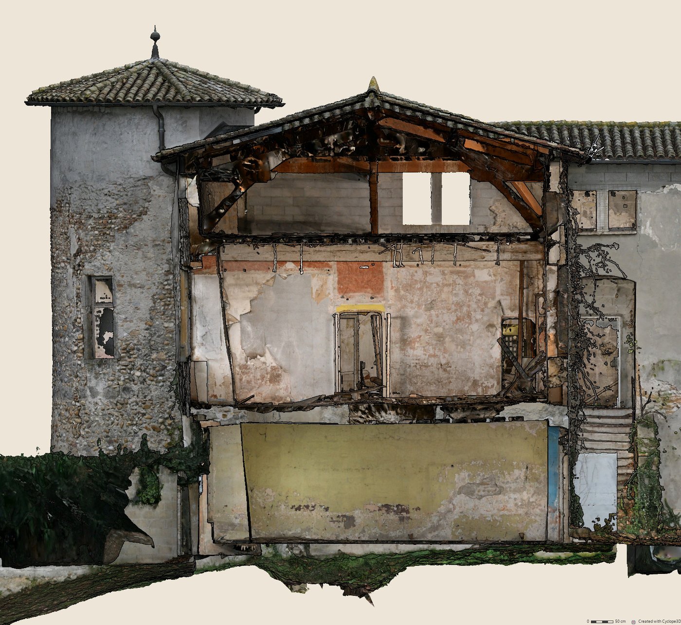
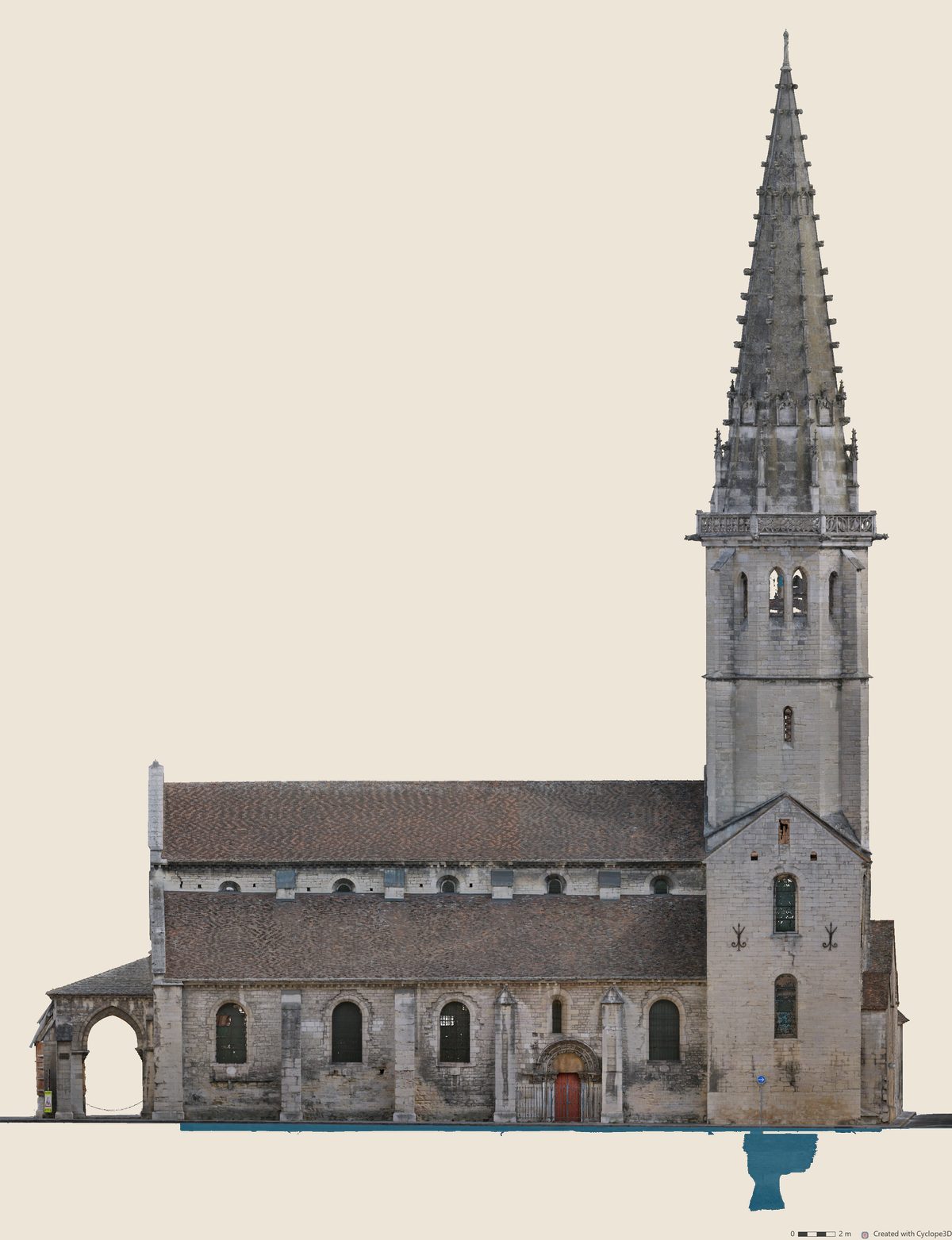
From the 3D model to AutoCAD drawings, with the default settings: one texture orthoimage per view, georeferenced, with its section line.
Opening the 3D model
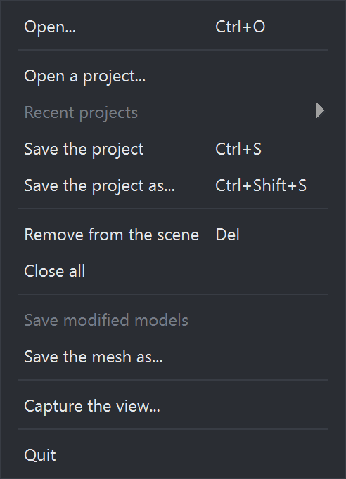
File > Open… menu (Ctrl+O), or a file dropped on the window: OBJ or PLY mesh, LAS, LAZ, E57 or PLY point cloud, 3DGS model. Every file opened is added to the scene.
Project name
Name typed in the first Name field of the Drawing outputs panel, for example
2609_stPhilibert. It prefixes every view folder and every file produced, followed by the type and name of the view.
Adding the views
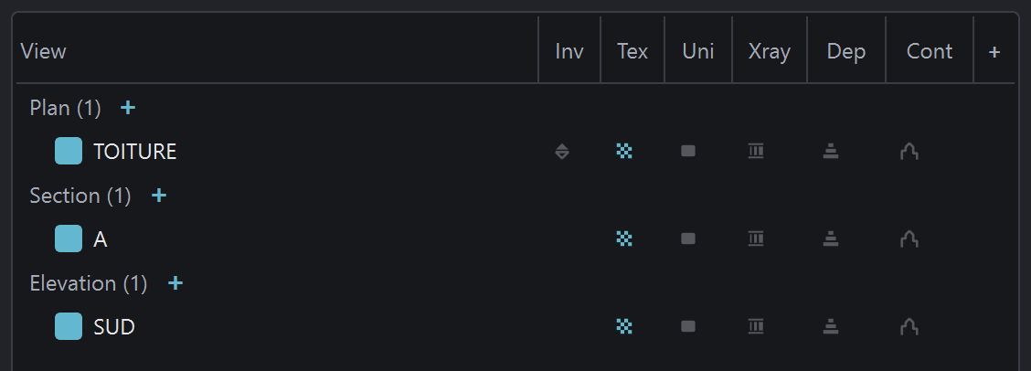
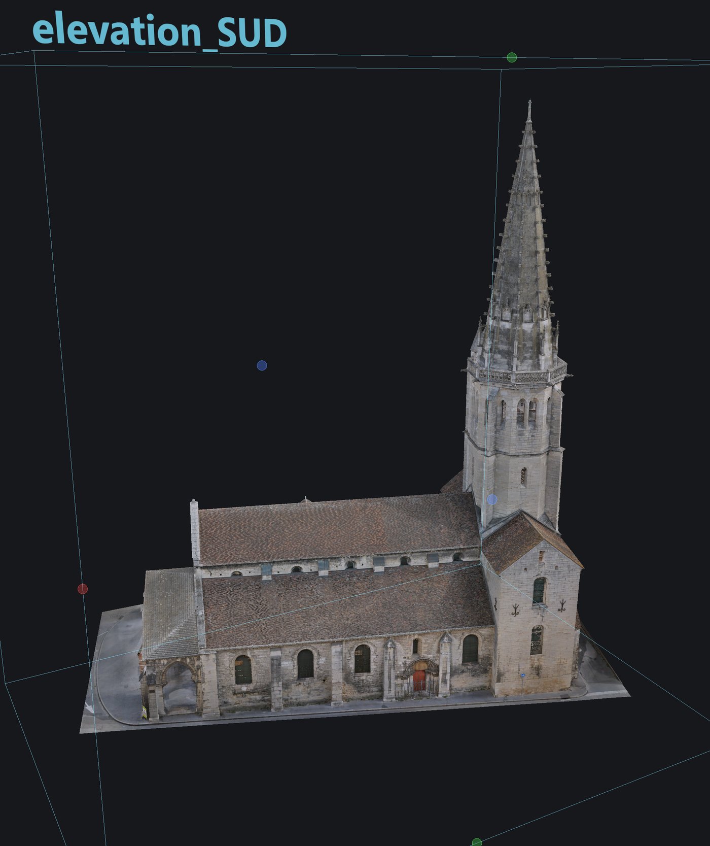
One “+” per family, in the list of views: plan, section, elevation. Every new view fits the extent of the model: a plan sits above it, as a roof plan; a section cuts through the middle of the model; an elevation shows the South facade.
Placing each view
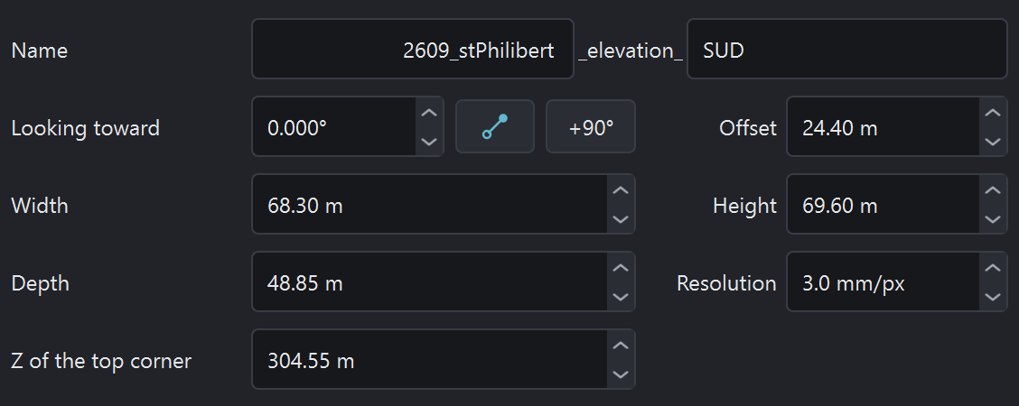
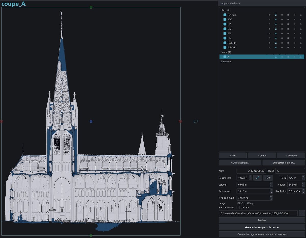
View selected in the list: its frame and handles appear in the 3D view, and the clipping box fits its volume. The handles are dragged with the mouse; the form gives the exact values: Looking toward, Offset (Height on a plan), Width, Height, Depth, Resolution.
Preview puts the camera on the axis of the view: the screen shows the image that will be extracted.
DWG conversion
Also convert the drawing to .dwg (ODA) box, in the Settings panel, Drawing outputs group. Every view then gets its drawing as DWG, next to the DXF. The setting is kept from one session to the next.

Generation
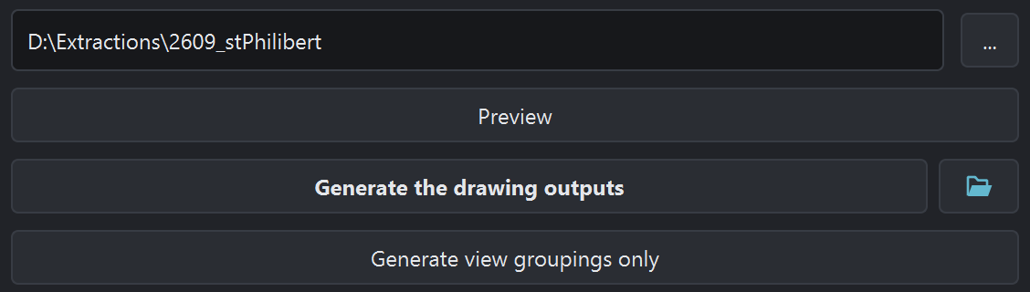
Output folder chosen with the … button, then Generate the drawing outputs. Every checked view gets its folder: the texture orthoimage and its world file, the section line, the DXF and DWG drawing, and a PDF sheet. The button on the right opens the output folder in the file explorer.
Result
2609_stPhilibert/
  2609_stPhilibert_elevation_SUD/   …
  2609_stPhilibert_plan_TOITURE/    …
  2609_stPhilibert_section_A/
    …_section_A.dxf · .dwg          drawing of the view
    …_section_A.pdf                 PDF sheet
    …_section_A__texture.jgw        its world file
    …_section_A__texture.jpg        texture orthoimage
    …_section_A_polyline.dxf        section line only
Advanced workflow with custom representations
Views placed to the centimeter, and extra orthoimages in the display of your choice: height or normals of a mesh; classification, intensity or slope of a point cloud. The steps come on top of those of the standard workflow.
Two-point orientation and height setting
Orientation by two points: the button to the right of Looking toward, then two clicks on the facade, from left to right, the way you read it standing in front of it. Z of the top corner sets the height of the top of the image: a round value makes the image land on a readable level.
Model coloring
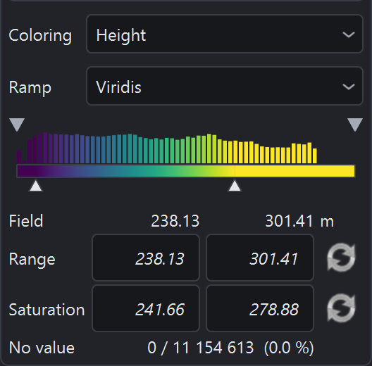
Model selected in the Scene panel, then the Coloring list: height or normals for a mesh; classification, intensity or a field computed by the Analysis menu for a point cloud. The ramp and the bounds, under the scale, set how the colors read.
Saving the representation
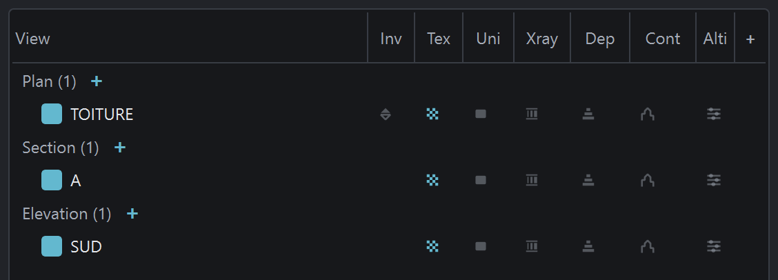
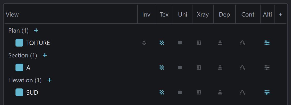
The “+” to the right of the Cont column saves the current display in a custom representation: color mode, ramp, bounds, classes, models shown, shading. Its column is added to the list of views; a double-click on its header renames it. Four representations at most.
Representation button
Every representation has its button in the rendering bar, after Depth: it brings the saved display back on screen. Its small dot saves the current display in place of the old one. The button stays lit as long as the scene matches.

Choosing the images per view
One dot per representation on every view row: lit, the image comes out at generation. A new representation arrives unlit on every view. A click on a dot of a selection applies to every selected view.
Engraved scale and groupings
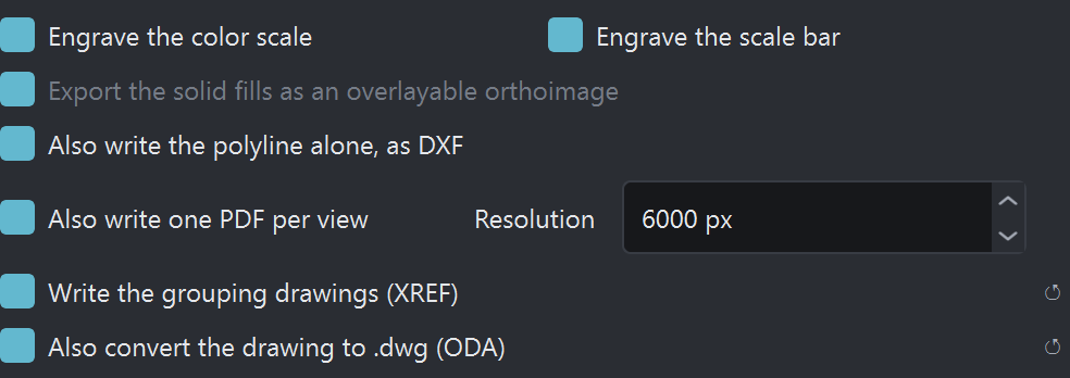
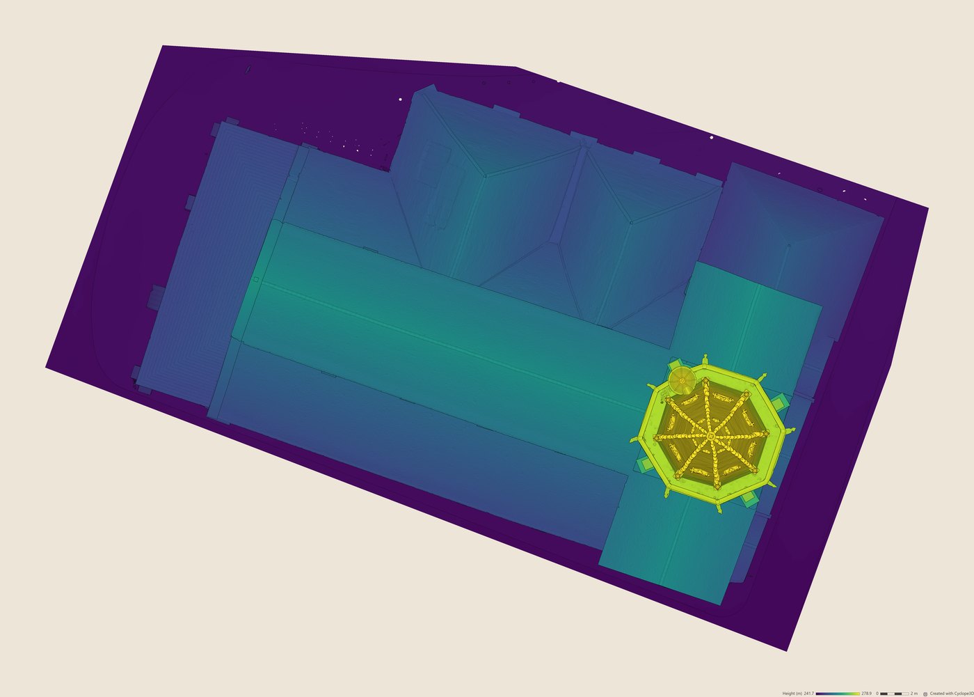
In the Drawing outputs group of the settings, Engrave the color scale writes the ramp used and its bounds into the image. Write the grouping drawings (XREF) puts at the root of the output folder one drawing of the plans and one of the elevations and sections, which call every view as an external reference, on its own layer.
Result
2609_stPhilibert/
  2609_stPhilibert_elevation_SUD/                            …
  2609_stPhilibert_plan_TOITURE/
    …_plan_TOITURE.dxf · .dwg                                drawing of the view
    …_plan_TOITURE.pdf                                       PDF sheet
    …_plan_TOITURE__Altitude.jgw                             its world file
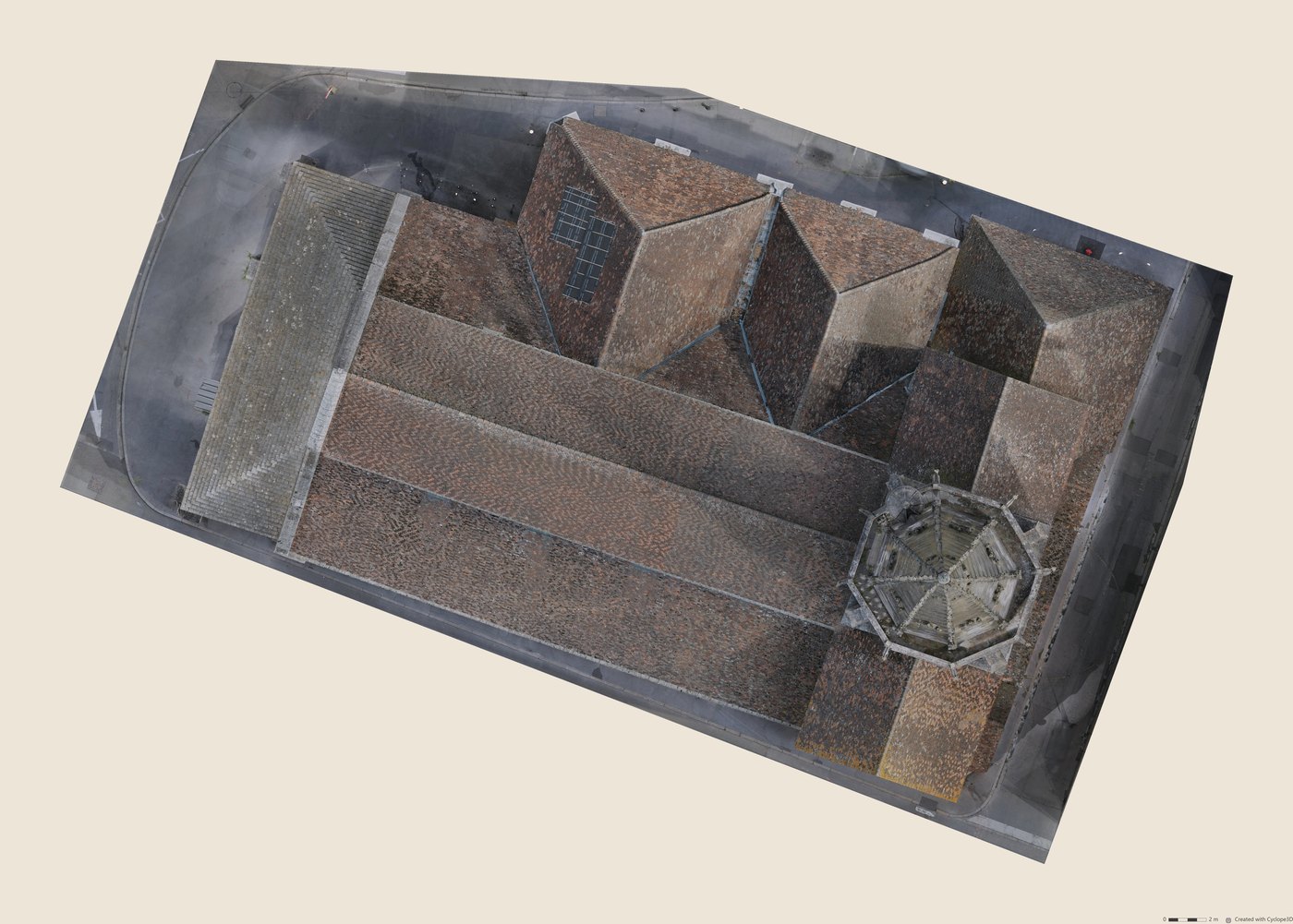
    …_plan_TOITURE__Altitude.jpg                             Altitude representation
    …_plan_TOITURE__texture.jgw                              its world file
    …_plan_TOITURE__texture.jpg                              texture orthoimage
  2609_stPhilibert_section_A/                                …
  2609_stPhilibert_position_elevations_sections.dxf · .dwg   place of elevations and sections
  2609_stPhilibert_position_plans.dxf · .dwg                 height of every plan
  2609_stPhilibert_regroup_elevations_sections.dxf · .dwg    elevations and sections, as external references
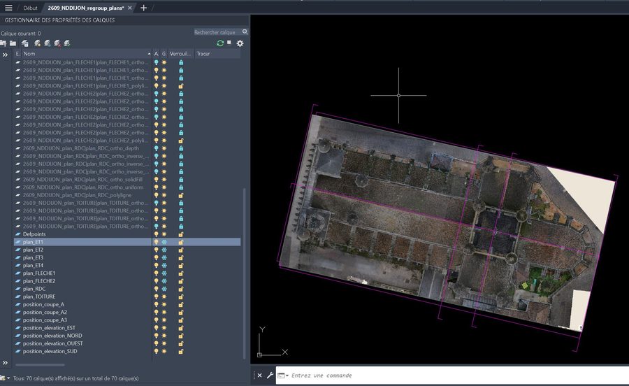
  2609_stPhilibert_regroup_plans.dxf · .dwg                  the plans, as external references
Inverse plan workflow (ceilings, vaults, roof structure)
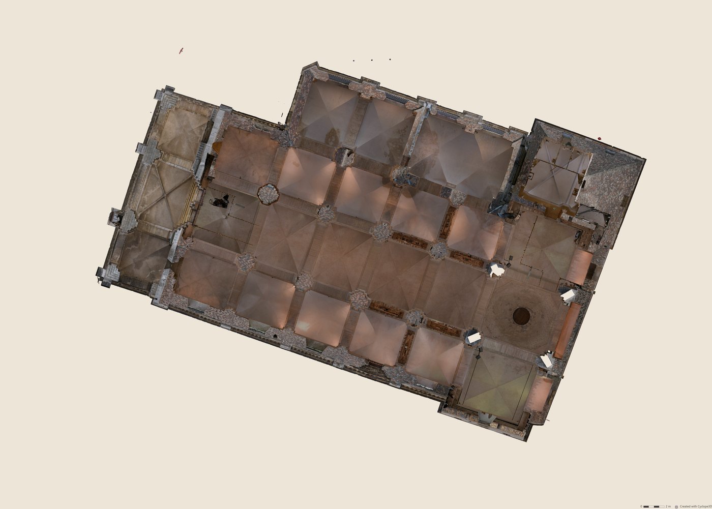
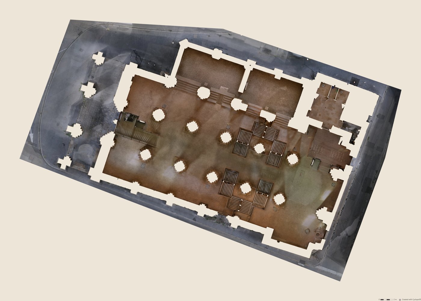
The inverse plan shows what lies above the cutting height of a floor plan: ceilings, vaults, roof structure, seen from below. It takes exactly the plan's rectangle, and the two images overlay in the drawing.
Floor plan
A plan added with the “+” of the Plan family, renamed in the last Name field (here
RDC), then lowered in the Height field to the cutting height: between 1 m and 1.20 m above the floor.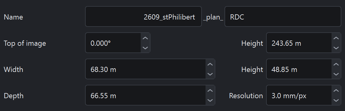
Checking the cut
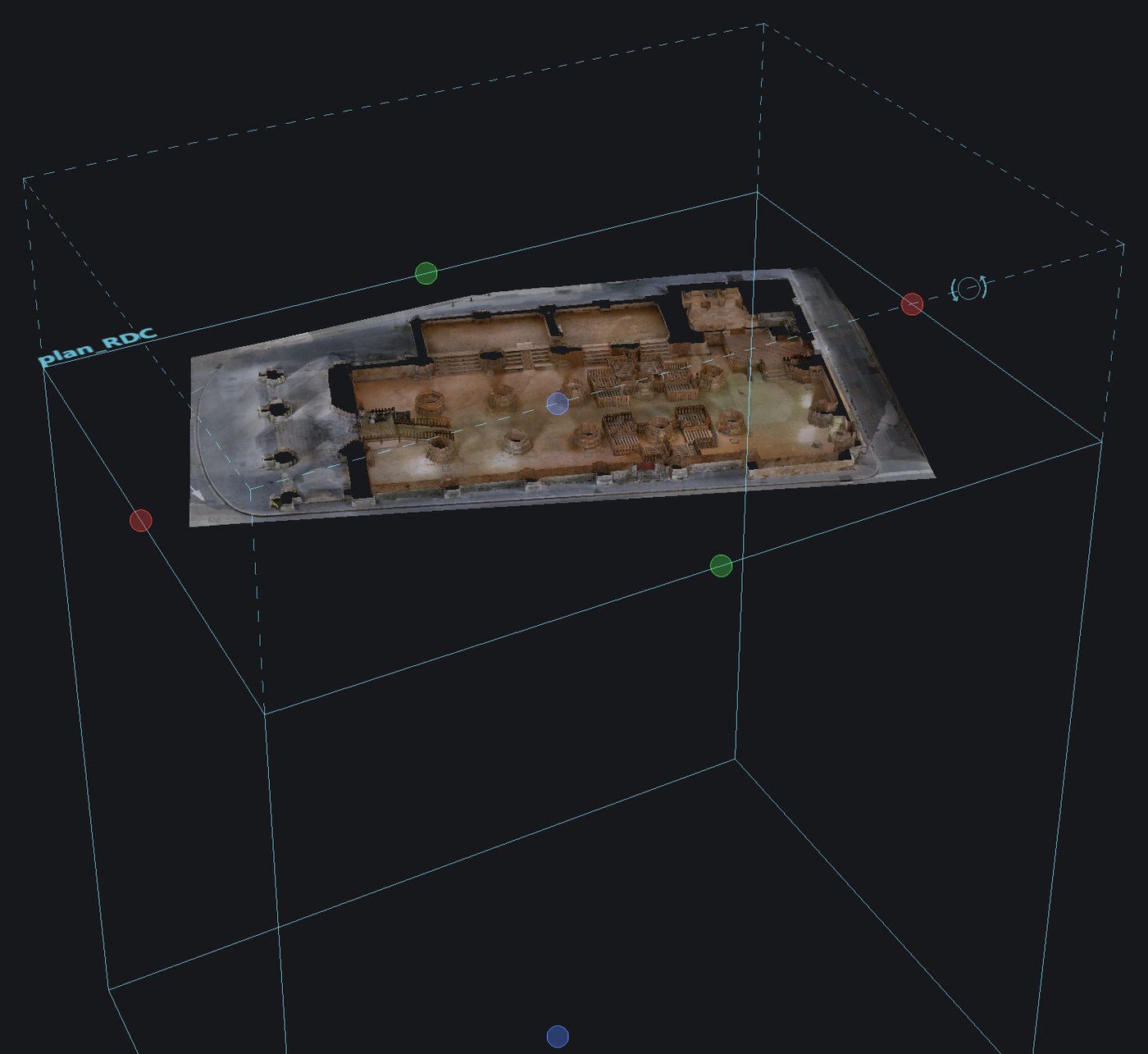
Plan selected in the list: the clipping box fits its volume, and the 3D view shows the building cut at that height, as the plan will draw it.
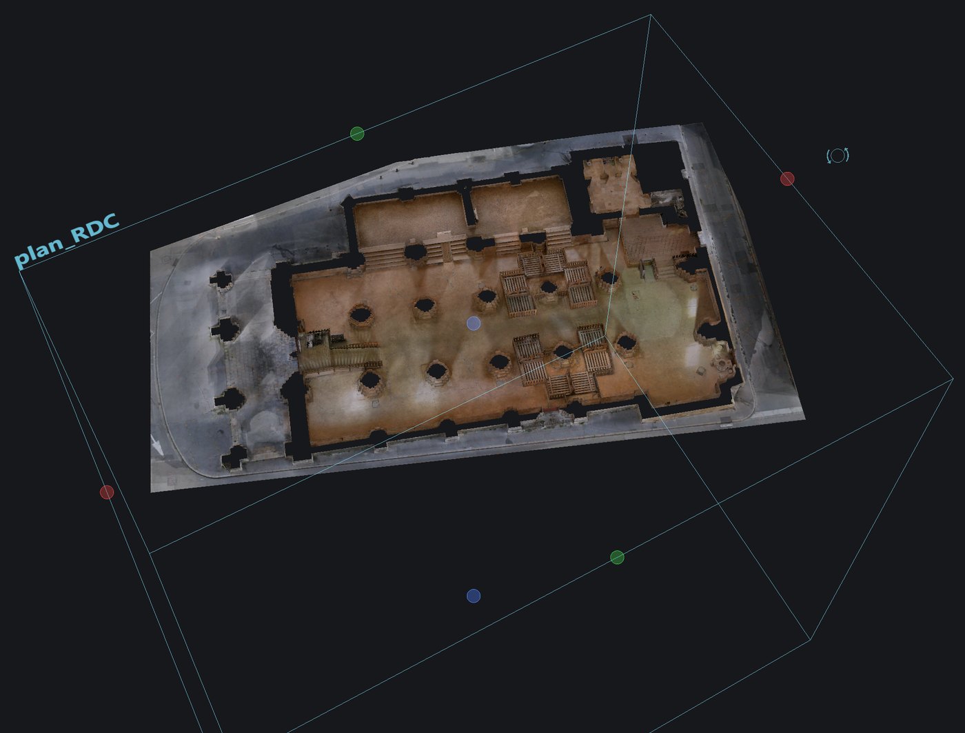
Inverse plan
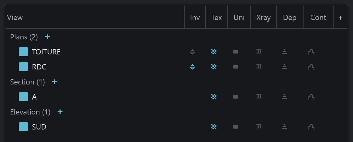
Inv dot lit on the plan row, in the list of views. The inverse plan takes the plan's rectangle (center, orientation, frame, resolution) and looks upward.
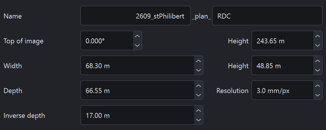
Inverse depth
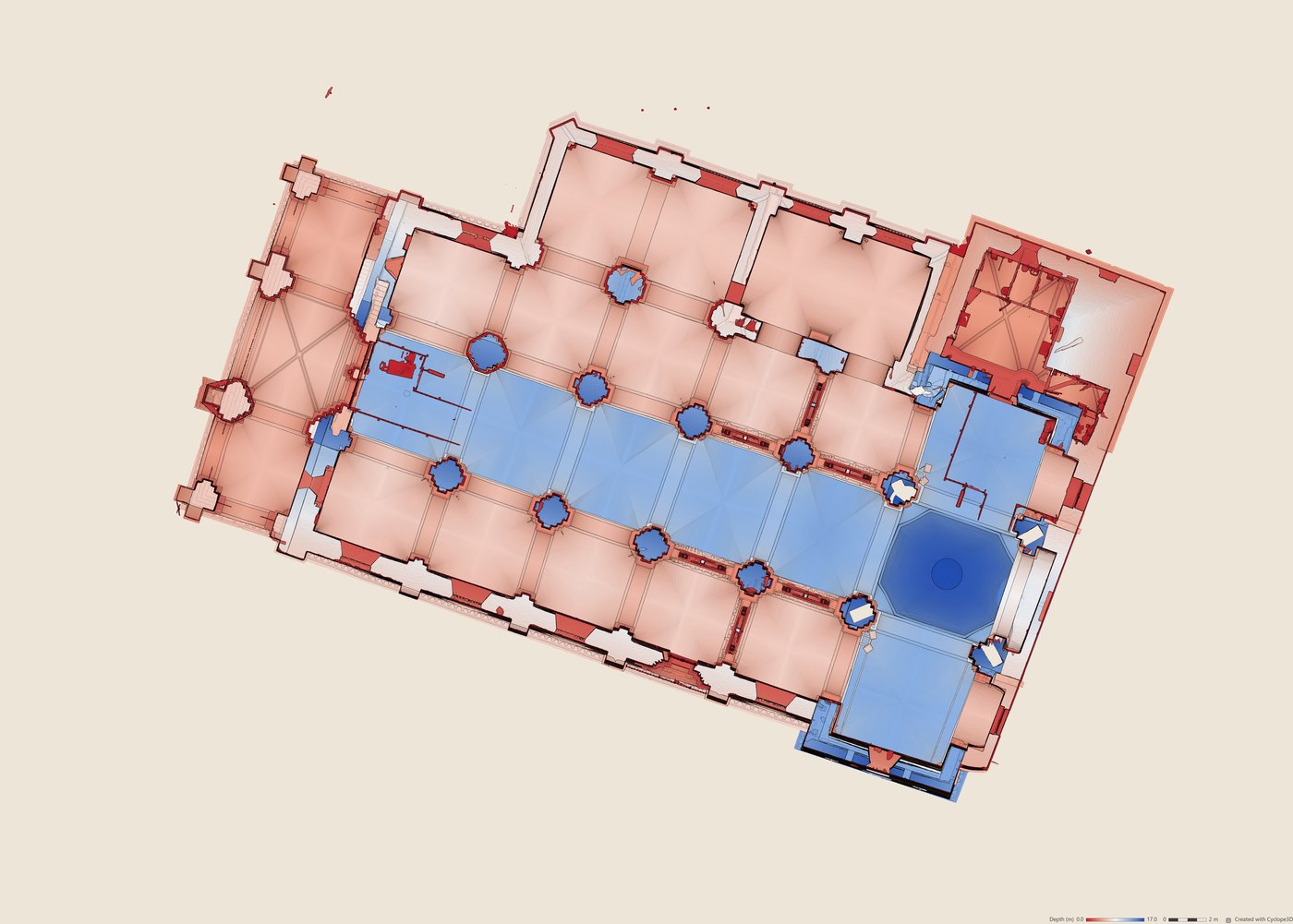
The Inverse depth field appears under Depth as soon as the dot is lit: the height the inverse plan sees above the plan, in meters. Default, No limit: ceilings, vaults and roof structure come out whole.
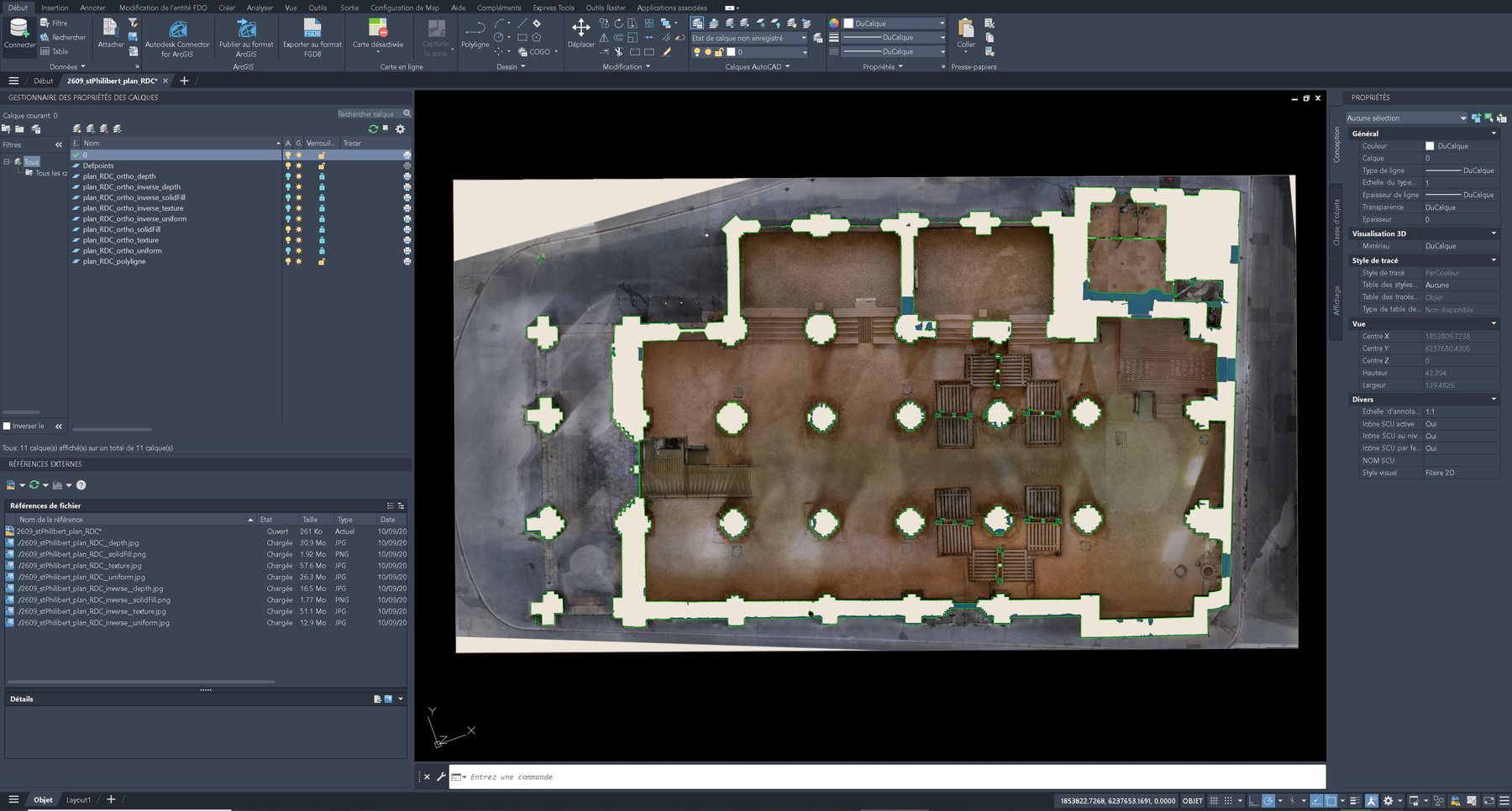
Here, 17 m: the nave vaults, whose keystones are 16.5 m above the cut, and nothing above.
Checking the volume
With the plan selected in the list, dashes show in the 3D view the volume the inverse plan sees: the plan's rectangle, raised by the inverse depth. With no limit, they rise to the top of the model.
Generation
Generate the drawing outputs: the plan's folder gets its images and those of the inverse plan, suffixed
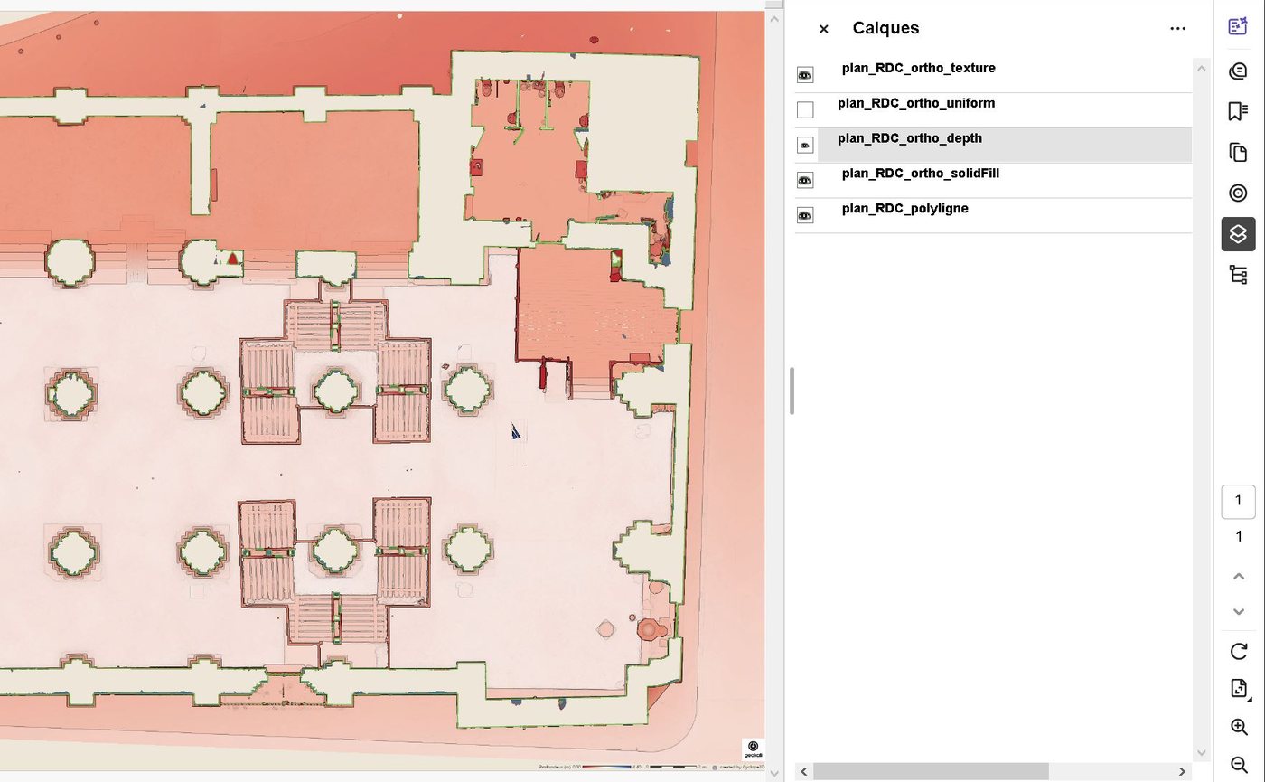
_inverse. A single drawing holds both, each on its own layer, with the plan's section line.Here, the row's Dep dot adds the depth map, for the plan and for its inverse plan.
Result
2609_stPhilibert/
  2609_stPhilibert_plan_RDC/
    …_plan_RDC.dxf · .dwg             drawing of the view
    …_plan_RDC.pdf                    PDF sheet
    …_plan_RDC__depth.jgw             its world file
    …_plan_RDC__depth.jpg             depth map
    …_plan_RDC__texture.jgw           its world file
    …_plan_RDC__texture.jpg           texture orthoimage
    …_plan_RDC_inverse__depth.jgw     its world file
    …_plan_RDC_inverse__depth.jpg     inverse plan, depth map
    …_plan_RDC_inverse__texture.jgw   its world file
    …_plan_RDC_inverse__texture.jpg   inverse plan, texture orthoimage
    …_plan_RDC_polyline.dxf           section line only
Workflow for clipping part of the model
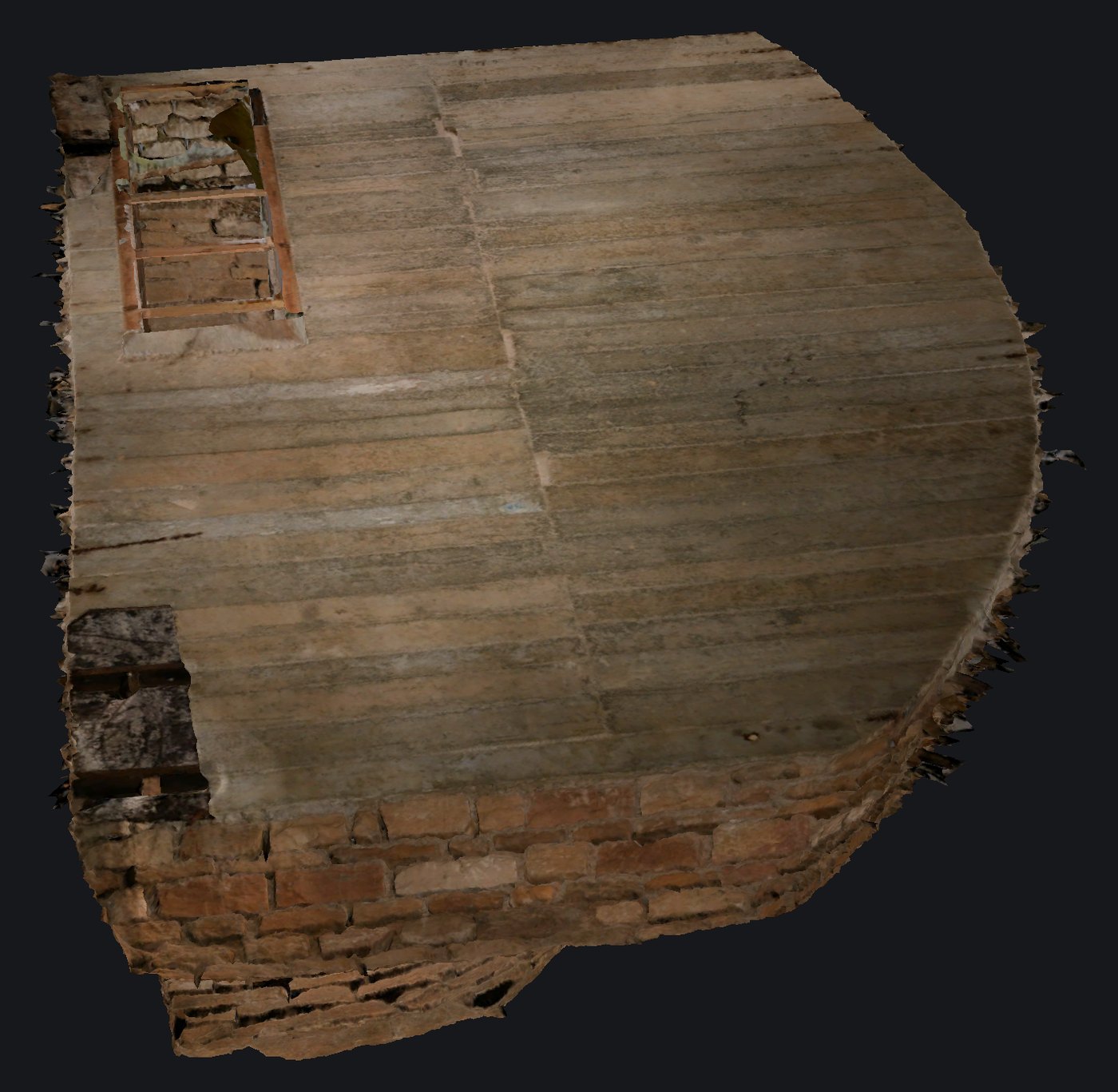
A part of the model isolated with the clipping box, to work on it alone: here the crypt of the Saint-Philibert church, under the church floor. The box only shows what it contains; Keep turns it into a separate model, cut clean at its faces.
Clipping box
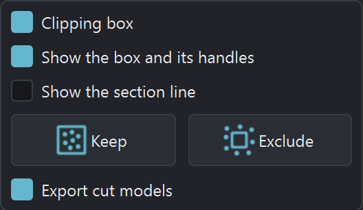
Clipping box box, in the panel of the same name, under the Scene list. Only what the box contains stays on screen.
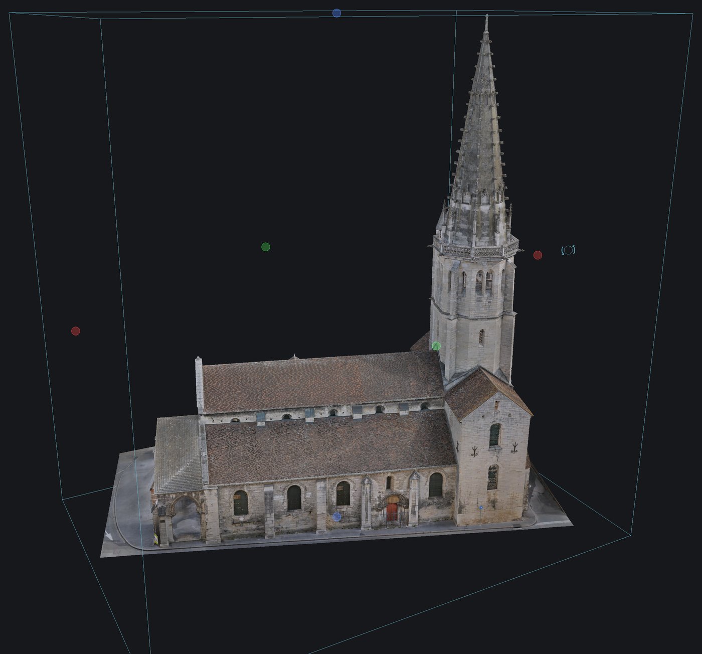
Box over the whole model
The box comes on over the whole extent of the model: here the whole church, before clipping, with the edges of the box and its handles. The crypt lies under the paving, out of sight from outside.
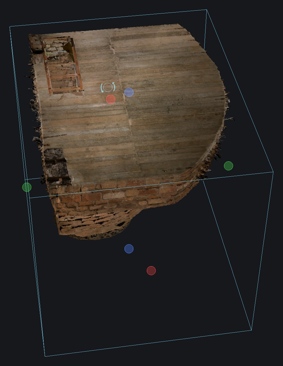
Setting the box faces
Every face of the box carries a dot in its middle: dragged with the mouse, it moves the face. The small ring on the side turns the box around the vertical, in line with the walls.
Here, the box hugs the walls of the crypt, 4.9 × 3.8 m, and its top face runs between the church paving and the plank ceiling of the crypt: the paving goes, the crypt stays whole.
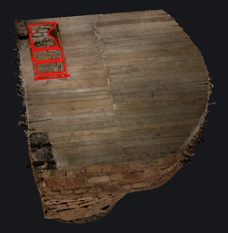
Checking the section line
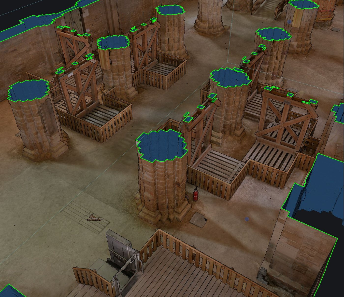
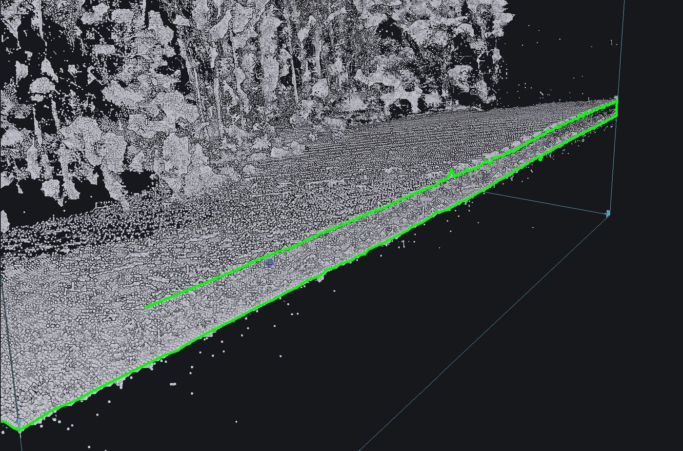
Show the section line draws the line where every face cuts through the material. With Show the box and its handles unchecked, the line stays alone with the model. On a mesh, it is redone at every move of the box.
Keep
Keep only retains from the models what the box contains: the mesh is cut clean at its faces, every triangle across a face cut again. Exclude does the opposite and removes what the box contains, a passer-by or a patch of sky for example.
Confirmation
A question states what becomes of every model, before any computation. OK: the cut model replaces its own in the scene, and the original file does not change. The box stays in place, ready for the next area.
Result
Groupings-only generation workflow
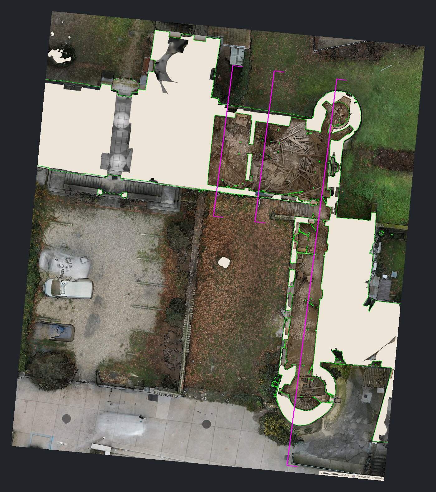
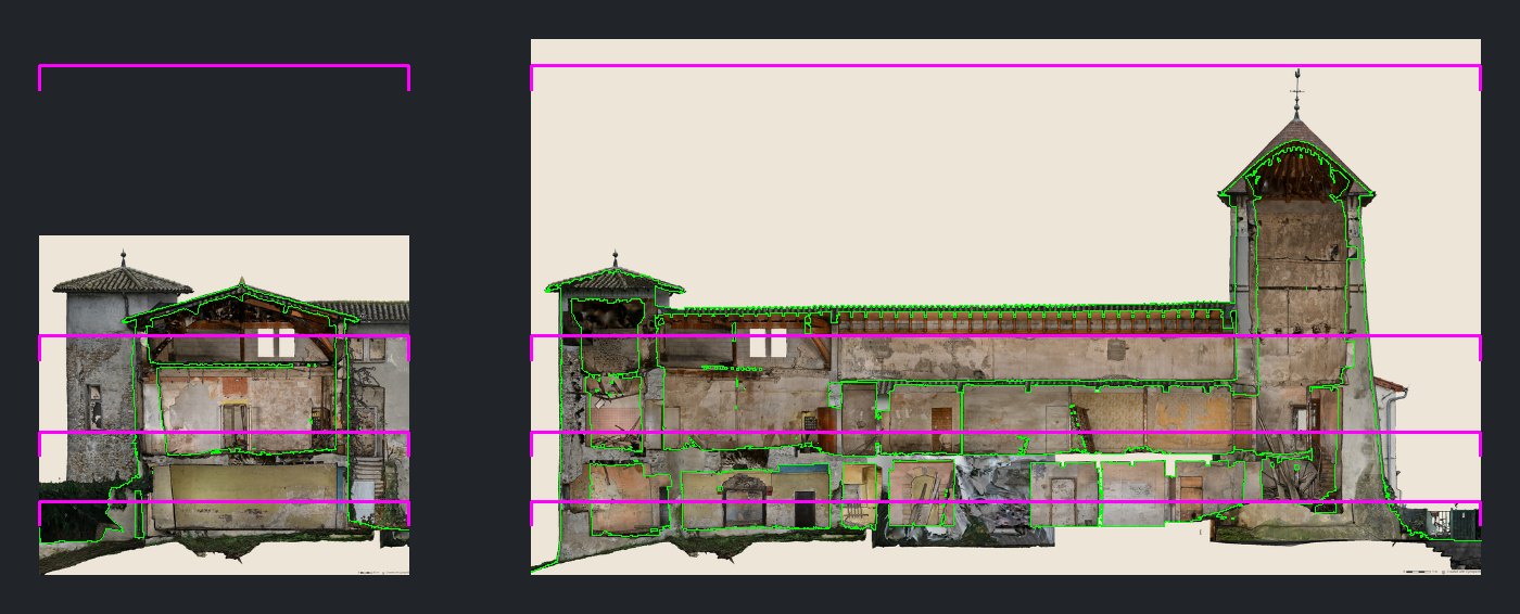
The groupings rebuilt from the drawings already generated, with nothing rendered: an extraction made in several goes, over several sessions or under several project names, is gathered at the end into one drawing of the plans and one of the elevations and sections. Example: the 2609_Vaux project, four plans and three sections.
Output folder
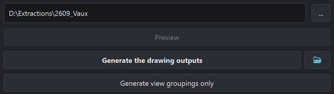
Output folder chosen with the … button: the one holding the view folders already generated. The project name, in the first Name field, prefixes the groupings. Neither views in the list nor a model in the scene are needed: the Generate view groupings only button is enabled as soon as a folder is chosen.
Choosing the drawings
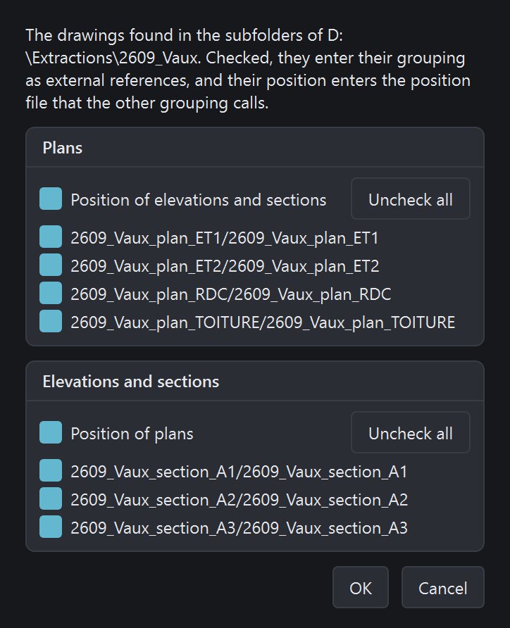
Generate view groupings only opens the View groupings window: the DXF and DWG drawings found in the subfolders, in two blocks, Plans and Elevations and sections. All arrive checked, those of another project too; the button of each block checks or unchecks the whole block.
On the line of that button, a box calls the position file of the other family: Position of elevations and sections in the Plans block, Position of plans in the other. It arrives checked; unchecked, the grouping does not call it, and the position file is still written at the root.
Writing the groupings
OK: four drawings are written at the root of the folder.
2609_Vaux_regroup_planscalls the plans, overlaid on their georeferencing;2609_Vaux_regroup_elevations_sectionssets the sections side by side, by orientation, at least 5 m apart. Each calls the position file of the other family: where the sections run on the plans, at what height the plans run on the sections.The report is shown under the buttons.

Result
2609_Vaux/
  2609_Vaux_plan_ET1/                                 …
  2609_Vaux_plan_ET2/                                 …
  2609_Vaux_plan_RDC/                                 …
  2609_Vaux_plan_TOITURE/                             …
  2609_Vaux_section_A1/                               …
  2609_Vaux_section_A2/                               …
  2609_Vaux_section_A3/                               …
  2609_Vaux_position_elevations_sections.dxf · .dwg   place of elevations and sections
  2609_Vaux_position_plans.dxf · .dwg                 height of every plan
  2609_Vaux_regroup_elevations_sections.dxf · .dwg    elevations and sections, as external references
  2609_Vaux_regroup_plans.dxf · .dwg                  the plans, as external references
Stacked sections and elevations workflow
Parallel sections of the same frame, stacked in the grouping: in AutoCAD, each one shows when its layer is thawed, on the same coordinates. Two sections, or an elevation and a section, are stacked when they look the same way and have the same frame; only the offset and the depth change. Example: sections A1 and A2 of the 2609_Vaux project.
Reference section
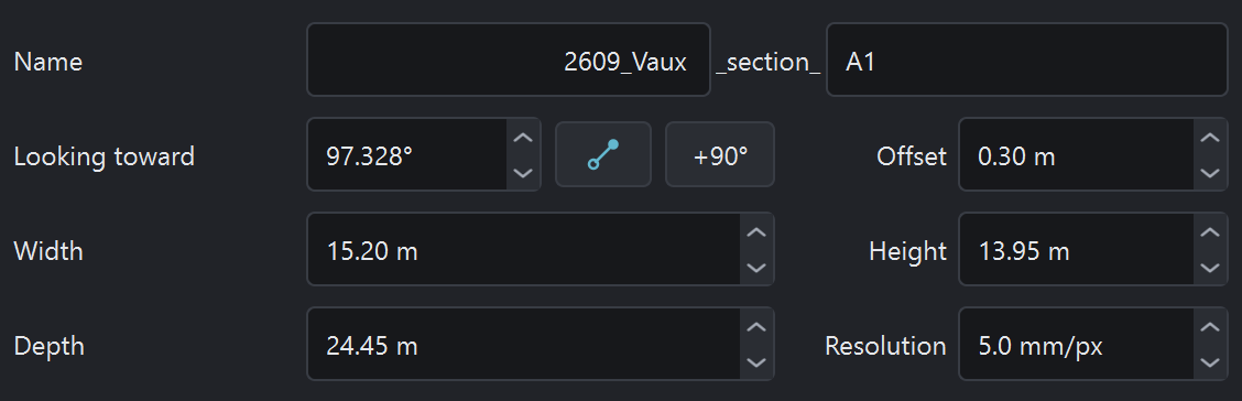
A section placed and framed, here A1: Looking toward, Width and Height, and its position in plan and in height, set with the handles. Stacked sections share this frame to the centimeter, and the viewing direction to a thousandth of a degree.
Duplication
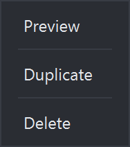
Right-click on the row of the section, in the list of views, then Duplicate: the copy takes the whole framing, gets the next name of the family and becomes the selected view.
Offset of the copy
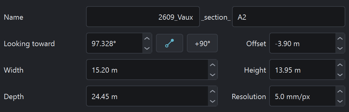
On the copy, here A2, only the Offset and, if needed, the Depth change. The offset goes from 0.30 m to −3.90 m: A2 cuts the building 4.20 m further along the viewing direction, in the same frame.
Stacked views
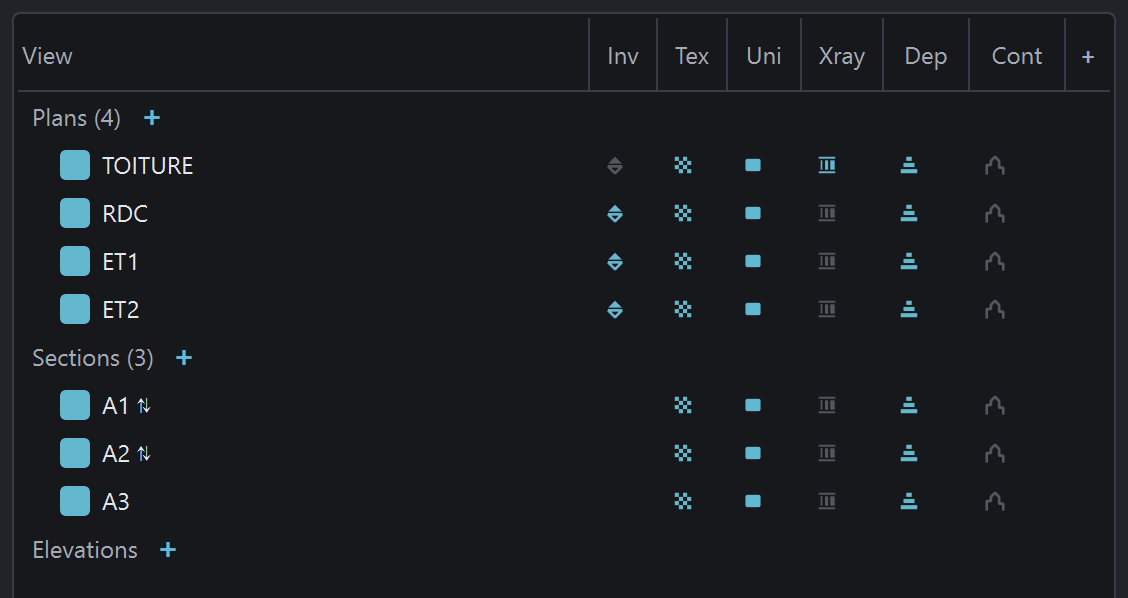
A ⇅ arrow follows the name of every stacked view, in the list. Its tooltip names the others: “Stacked in the grouping with section_A2: same viewing direction, same frame”.
Generation and grouping
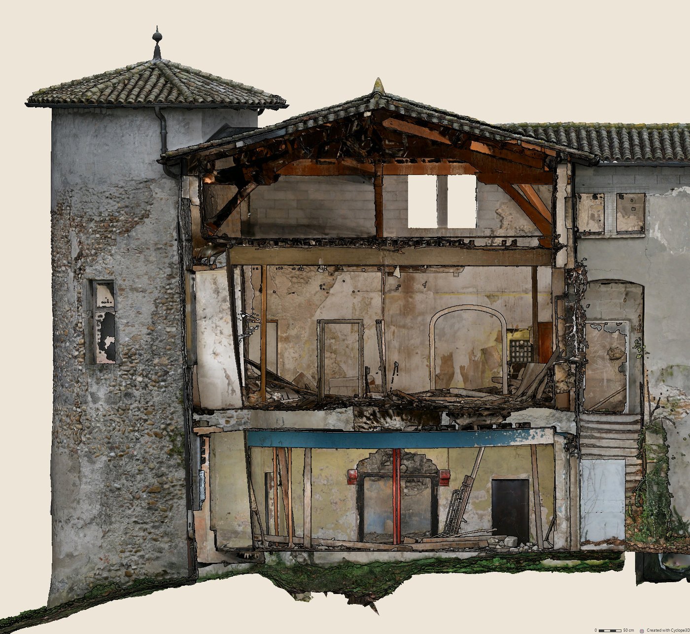
Write the grouping drawings (XREF) checked with the DWG conversion, then Generate the drawing outputs. In
2609_Vaux_regroup_elevations_sections, A1 and A2 share the same place, each on its own layer; A3, with another frame, sits 5 m further on.
Result
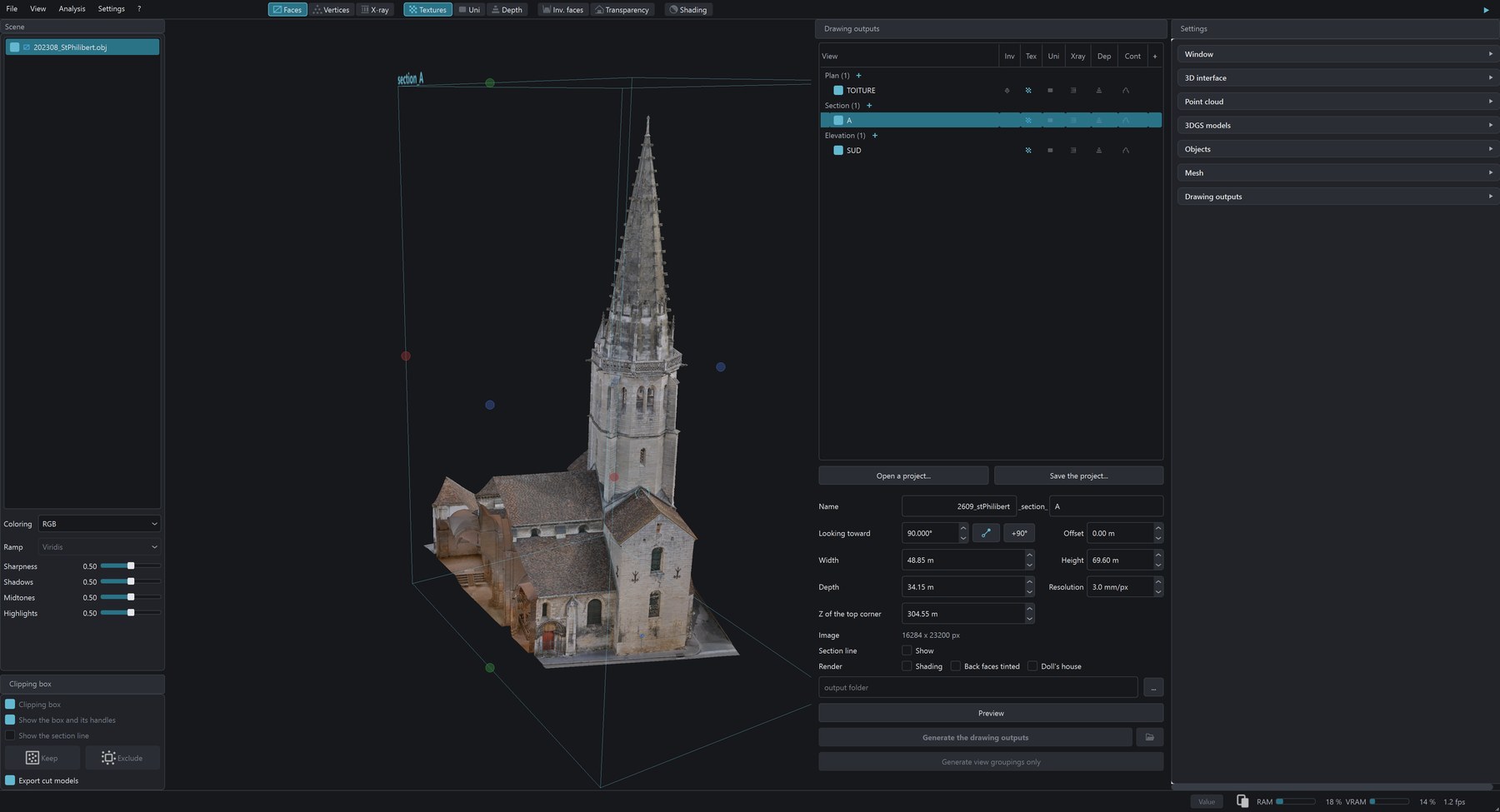
The software window
Rendering bar
Above the 3D view.

- Faces
Displays meshes as surfaces, with their texture or their flat tint. This is the usual display mode.
A 3DGS model shows its splats blended, as in the photos.
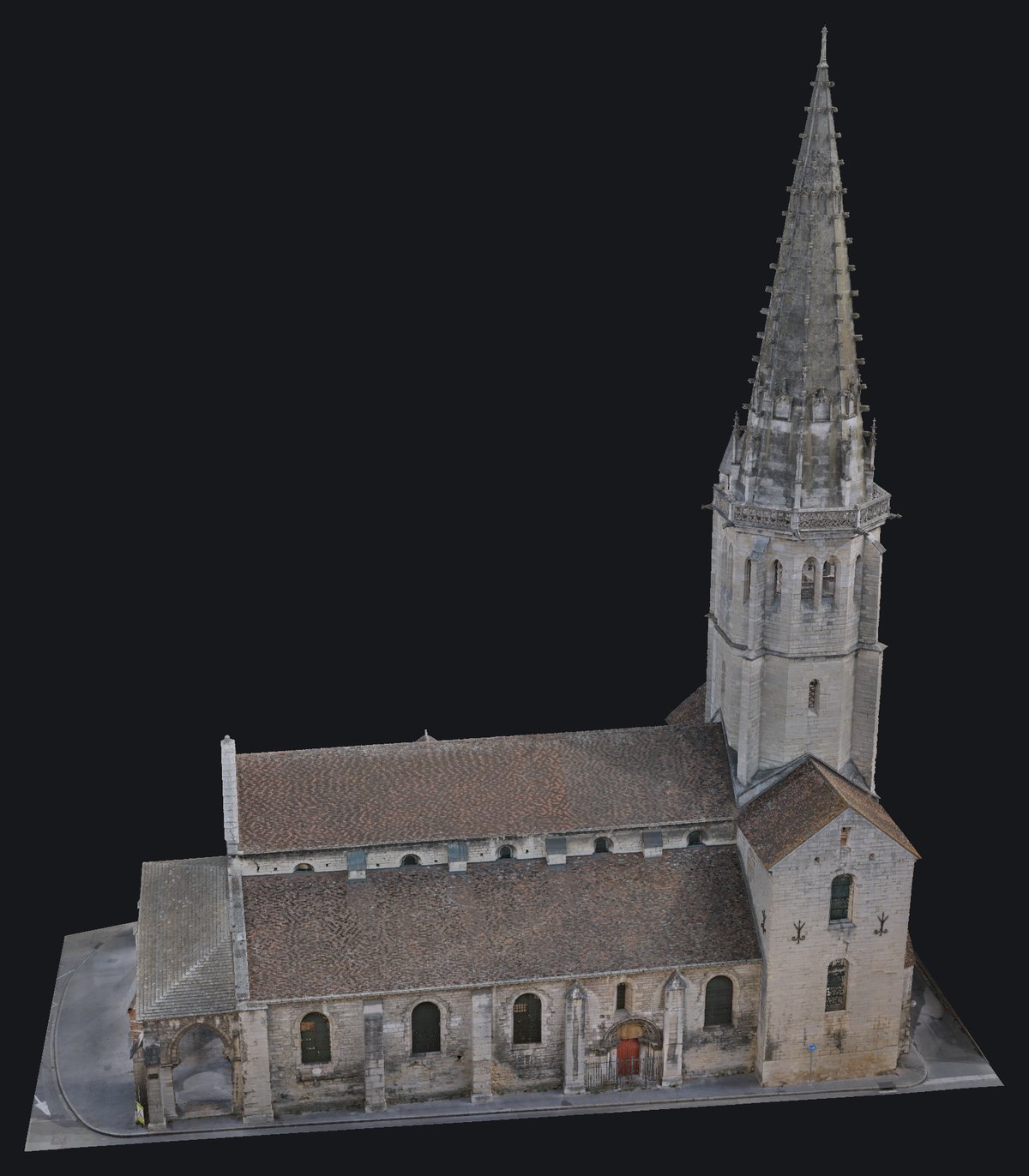
- Vertices
Displays mesh vertices as points, each with the color of its texture. For a 3DGS model, the center of each splat is shown.
A point cloud is always displayed as vertices: the button lights up as soon as a cloud is open, and leaves the X-ray.
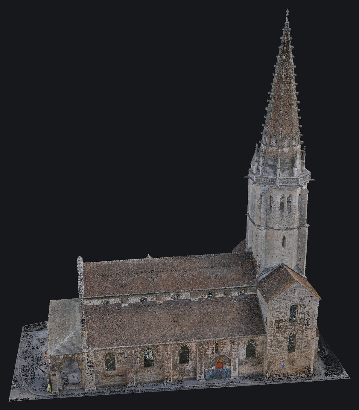
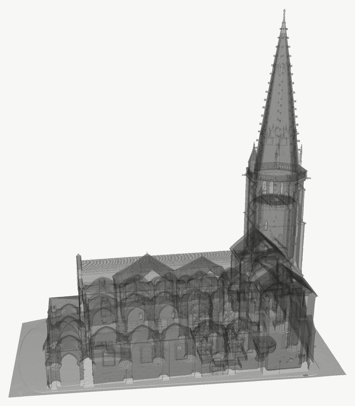
- X-ray
See-through rendering, like an X-ray, a third drawing mode after the faces and the vertices: everything the ray crosses accumulates, so you can see through the material, for example services behind a false ceiling or the furniture behind a wall.
A surface seen edge-on weighs more than one seen face-on, in the manner of MeshLab: walls and frames stand out, large flat areas fade. Works on meshes, clouds and 3DGS models.
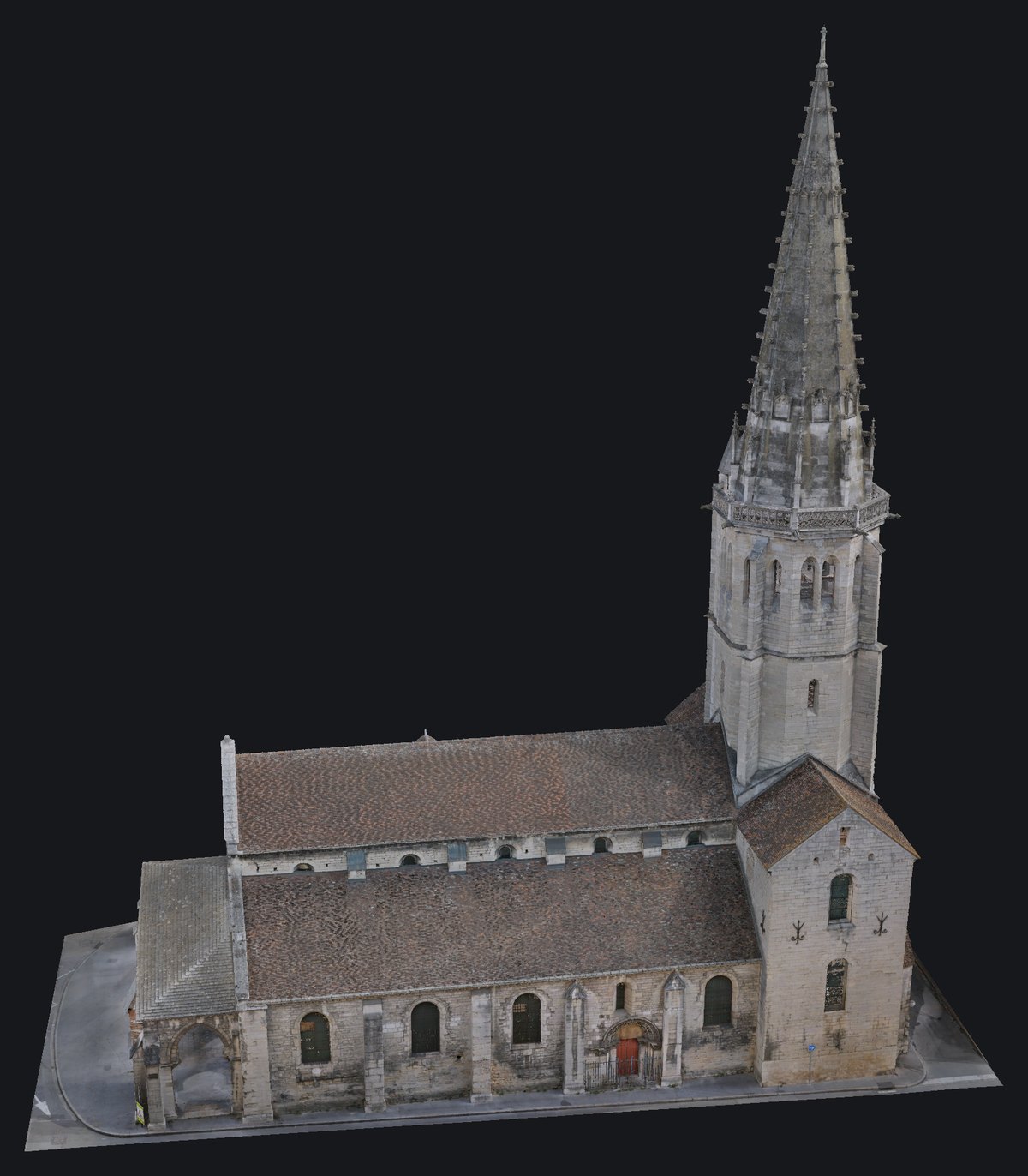
- Textures
Displays the models' own color: the photo draped over meshes, the RGB color of points on clouds. 3DGS models keep their reflections, which change with the viewing angle.
A cloud without color keeps the field it is showing.
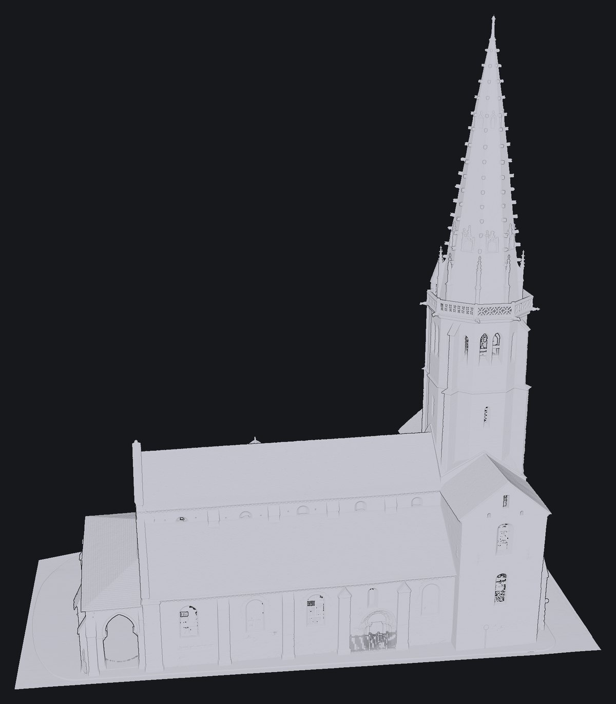
- Uni
Displays all models in a flat tint, without their photo, to read the shape rather than the material. The tint is set in the settings (Uniform color).
A cloud colored by a field, such as height, also switches to the flat tint; its field is picked again in the Scene panel. Switching back to textures is immediate.
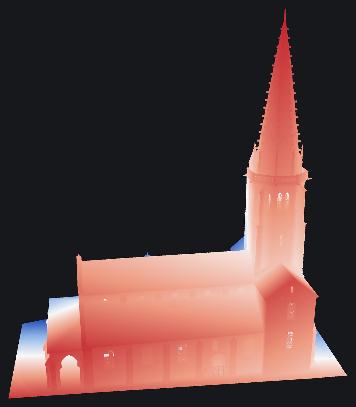
- Depth
Colors the models by their distance, from red for the nearest to blue for the furthest, with the same ramp as the depth maps of the orthoimages.
With a view selected in the drawing outputs, the distance is counted from that view's plane: the screen shows the depth map that will be delivered. With no view selected, the scale adapts to what is visible on screen.
- Inv. faces
Displays the back of faces in a dark tint. Open volumes then read as hollow, which reveals the gaps in a survey. The tint is set in the settings (Back-face color).
Also applies to clouds whose normals are oriented, and to 3DGS models once the splat directions are computed (Analysis > Splat directions).
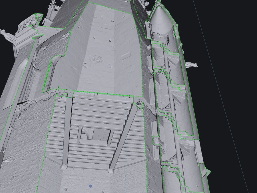
Back faces left as they are 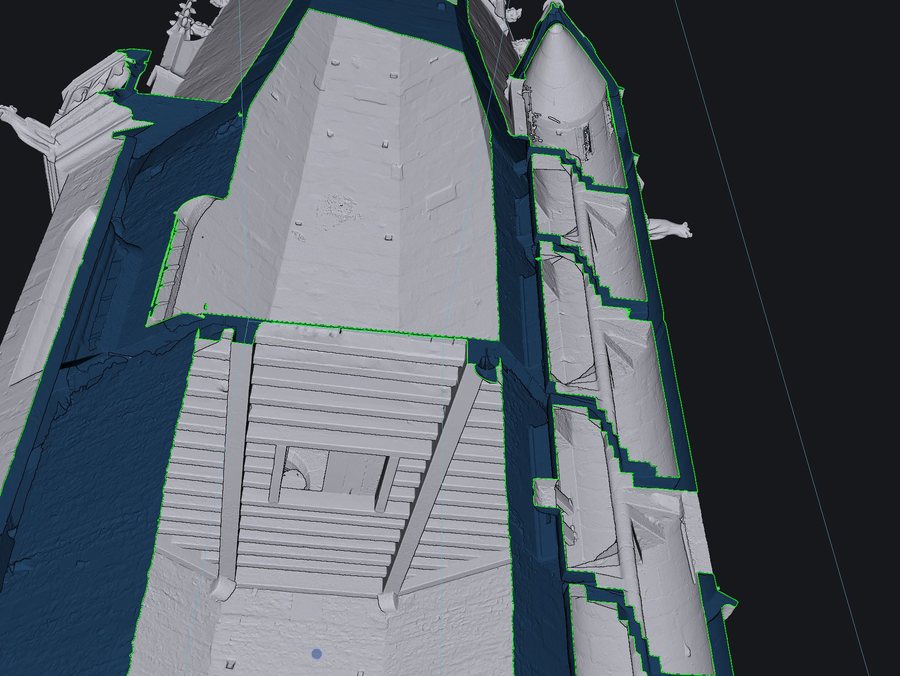
Back faces tinted - Transparency
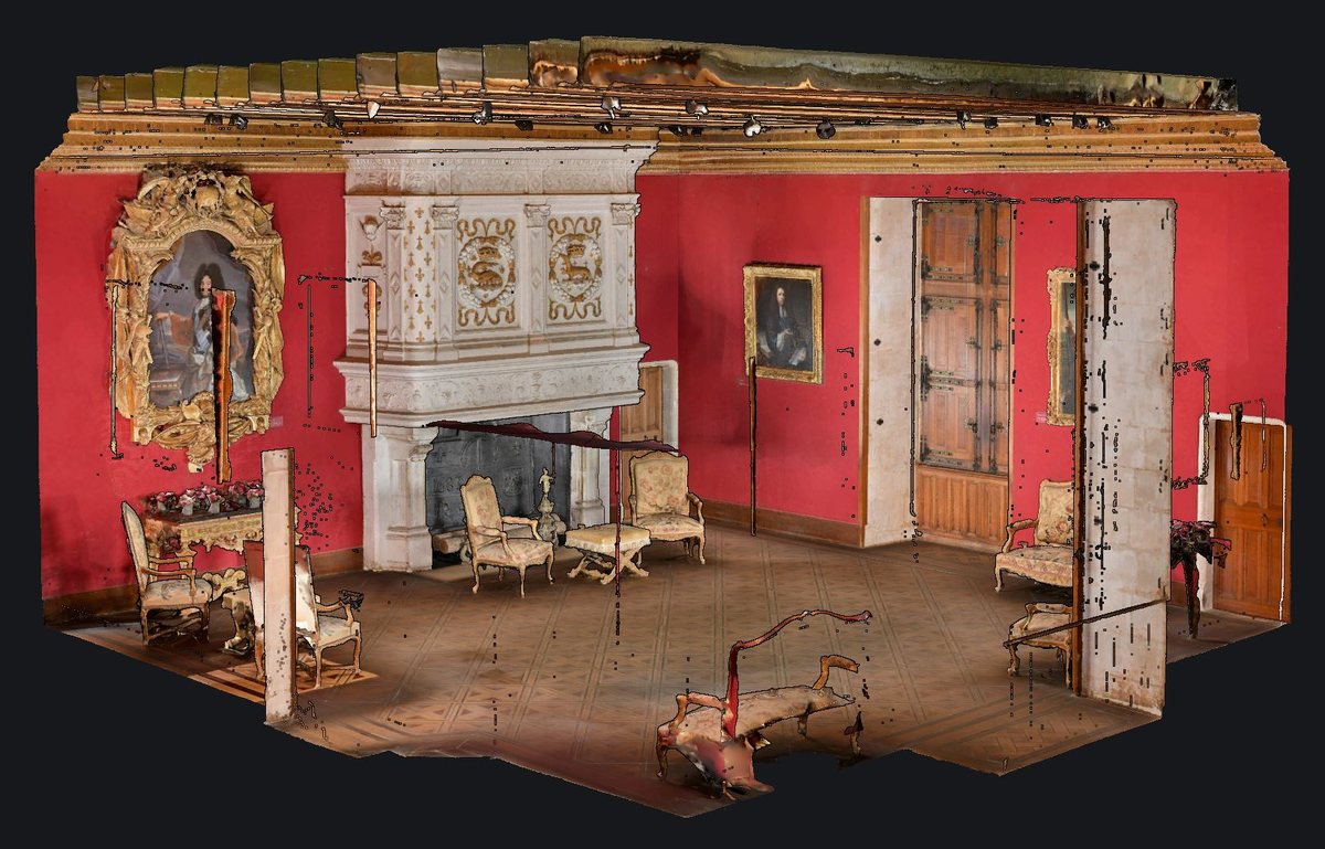
Hides the faces turned away from the camera, as in a dollhouse. On an interior survey seen from outside, the nearest wall disappears and you see into the room.
An exterior survey does not change, apart from its inside-out faces, which show as holes. 3DGS models need the splat directions (Analysis > Splat directions).
- Shading
EDL shading (eye-dome lighting), which darkens hollows and depth breaks. It brings out the relief of a dense cloud without color; on a photogrammetric texture, already lit, it adds little.
Its strength is set in the settings. Orthoimages follow this button: when it is on, the extraction shades its images with the same strength.
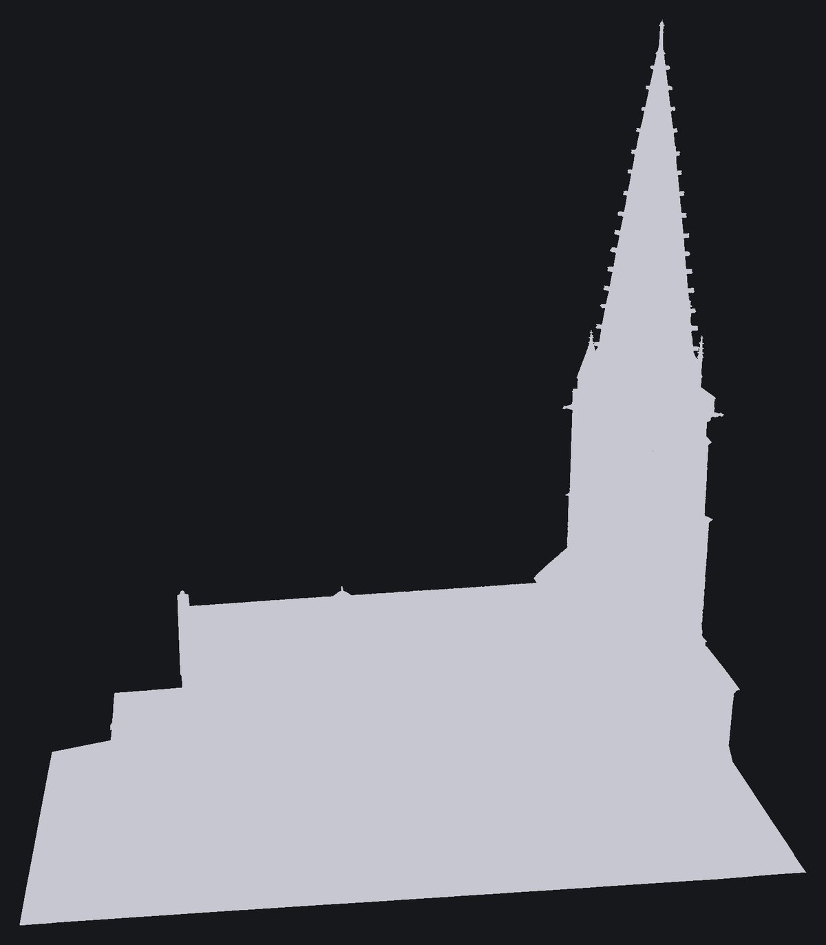
Without shading With shading
Status bar
Below the 3D view, with the pivot coordinates.

- Value
Reads the value of the displayed field at the cloud point nearest the pivot, that is, the point set by the last double-click.
The search runs through the whole cloud: instant on a small survey, it takes a few seconds on a very large one. That is why it runs on demand.
- Copy the pivot
Copies the pivot coordinates to the clipboard: X, Y and Z to the millimeter, in the file's coordinate system, and the field value if it has been read.
- Cancel
Stops the running computation or loading (Esc key). Nothing already computed is kept, and a canceled loading also drops the files waiting in line.
Scene panel
The open models, and the coloring of point clouds and meshes.
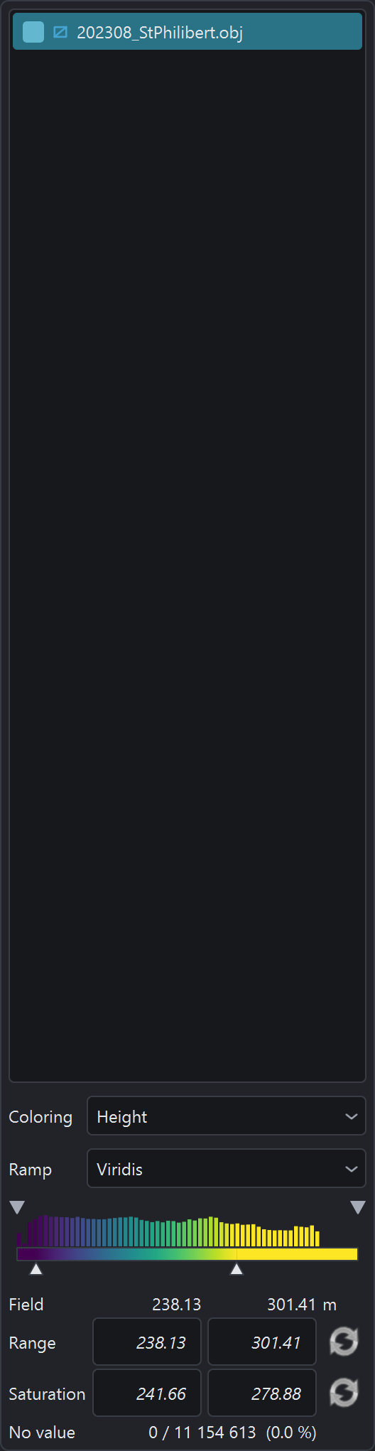
- Model list
List of the open models. For each model:
- checkbox: show or hide, without unloading;
- double-click: reframe the view on the model, or reload it if it was unloaded;
- Del: remove the model from the scene and free the memory;
- right-click: file information, grouping several models under one name, unloading from memory while keeping the row;
- drag: change the order of models or groups.
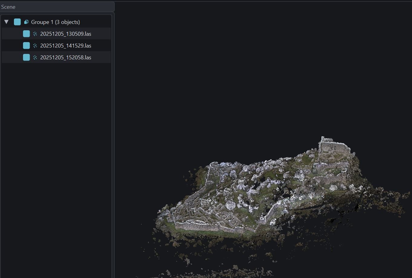
- Coloring
Chooses what the color represents: RGB color, flat tint, or a field of the model (height, intensity, classification, computed fields…).
Applies to the selected clouds and meshes, or to all clouds if nothing is selected.
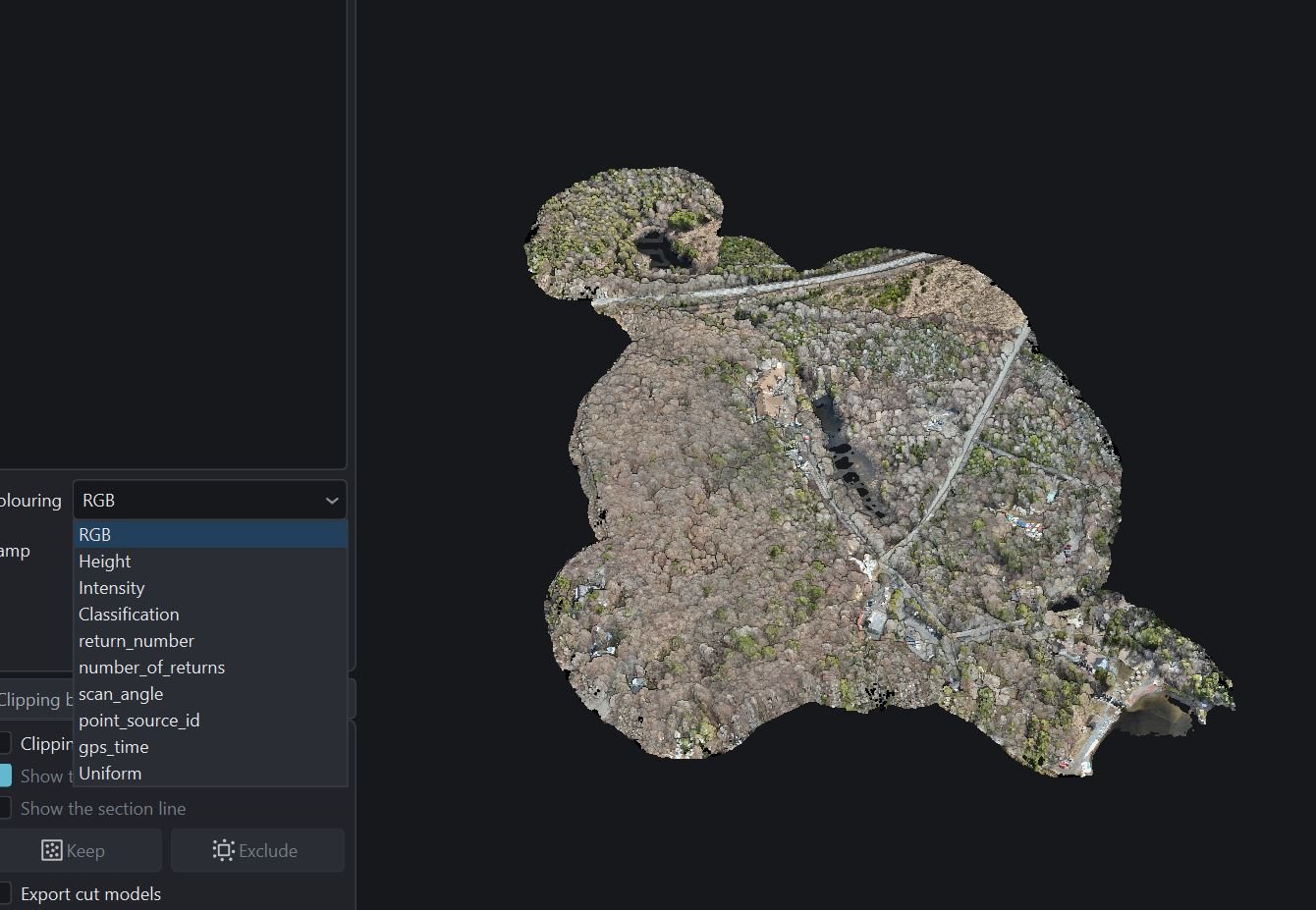
- Ramp
Color palette applied to the displayed field:
- Viridis: even and readable with color blindness, the safest choice;
- Blue-green-yellow-red: CloudCompare's, to get the same images from one program to the other;
- Green-red: for a quantity that is judged, such as a sheet thickness;
- Blue-white-red: for a signed quantity, on either side of zero.
- Point classes
List of the classes present in the cloud, with the ASPRS standard names. An unchecked class becomes points with no value: its points show in the flat tint, or disappear if the Points with no value box is unchecked.
- Sharpness
Sharpness of the model's own colors: RGB of clouds, photo of meshes, 3DGS splats. To the right, edge contrast increases, with no halo along the joints; to the left, the image softens. Default 0.5: no change.
- Shadows
Adjustment of the shadows of own colors. To the right, they lighten: black rises up to a quarter; to the left, they block up. Default 0.5: no change.
- Midtones
Adjustment of the midtones of own colors, through the gamma. To the right, they lighten; to the left, they darken. Default 0.5: no change.
- Highlights
Adjustment of the highlights of own colors. To the right, white is reached from three quarters; to the left, the lights dull. Default 0.5: no change.
- Coloring scale
Scale of the displayed field, with its histogram:
- the arrows at the top bound the displayed range: beyond it, points have no value;
- the handles at the bottom bound the saturation: beyond it, points keep the color of the end of the ramp;
- a double-click on a row sets it back to automatic.
The histogram uses a logarithmic scale, so that isolated values stay visible.
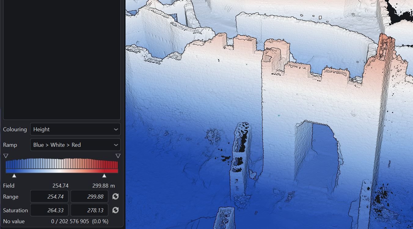
- Field
Smallest and largest values actually present in the field, outliers included.
- Range
Bounds of the displayed range. Points outside it have no value: they take the flat tint, or are hidden with the Points with no value box.
In italics, the range follows the field. Type a value to fix it, empty the box to go back to automatic.
- Saturation
Bounds of the color ramp. Points beyond them keep the color of the end and stay displayed.
In italics, they follow the field. Type a value to fix them, empty the box to go back to automatic.
- No value
Number of points with no value (holes in the field, points out of range), out of the number of colored points.
Clipping box panel
The box that limits the scene, and model cutting.
- Clipping box
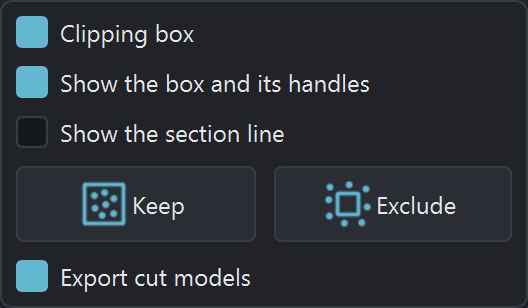
Limits the display to what lies inside the box. Parts entirely outside are no longer drawn at all, which also lightens the load on the graphics card.
The box is set with the mouse in the 3D view: a handle in the middle of each face to pull it, a ring on the side to turn it about the vertical.
- Reset the box
Resets the box to the extent of the scene, level. The box stays on or off.
- Show the box and its handles
Shows the edges and handles of the box. Unchecked, the clipping still acts but the box is no longer drawn: handy to judge the result, or to take a clean screenshot.
- Show the section line
Shows the line where each face of the box cuts the material, in the color and width of the drawing outputs' section line. On screen only: nothing is written to the files.
- Keep
Keeps only what lies inside the box. Meshes are cut clean at the faces of the box; a model the box does not touch stays intact.
The cut model replaces the original in the scene. The original files are never changed.
Before 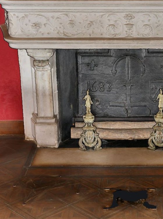
After - Exclude
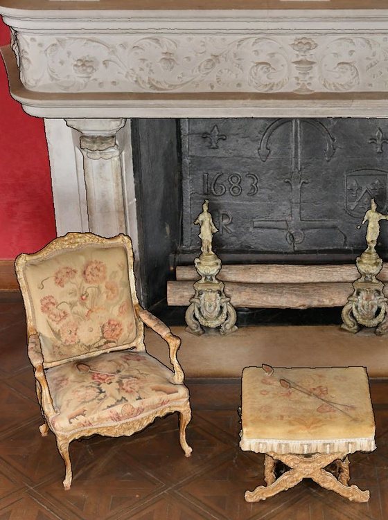
Removes what lies inside the box: a stray point, a passer-by, a patch of sky. Meshes are cut clean at the faces of the box, which then turns off to show the result.
The cut model replaces the original in the scene. The original files are never changed.
- Export cut models
Checked, Keep and Exclude write each cut model to a new file (LAS, PLY or OBJ), next to the original. Unchecked, the cut stays in memory, in italics in the Scene list.
Drawing outputs panel
The views to extract—plans, sections and elevations—and the form of the selected view.
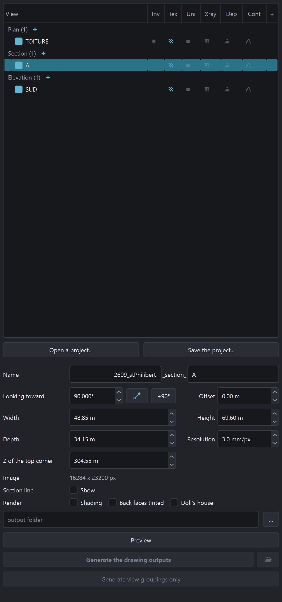
- View list
List of the views to extract, sorted into plans, sections and elevations:
- checkbox: the view goes to extraction, or stays in reserve;
- “+” of a family: add a view;
- double-click: put the camera on the axis of the view;
- Del: remove the selected views;
- drag: change the order; a section can become an elevation, and the other way round;
- dot to the right of a plan: also extract the inverse plan, seen from below.
- Add a plan
Adds a plan: a view of the model from above, cut at the chosen height. The matching inverse plan (ceiling, roof frame) can be added to the same drawing.
- Add a section
Adds a section: the plane of the view cuts through the model, and you see what lies behind it. It is also the view to use for a room wall seen from inside.
- Add an elevation
Adds an elevation: an exterior view of a facade, from the side it is looked at from.
- Open a project…
Opens an extraction project (
.extracts): every view with its position, orientation, frame and resolution, and the output settings. The project's views replace those in the list.- Save the project…
Saves the extraction project (
.extracts), to make exactly the same images again later, for example after the mesh has been reworked or the resolution changed.- Project name
Prefix of every file produced, also used as the AutoCAD drawing name. A view named RDC in the project 2609_stPhilibert thus gives
2609_stPhilibert_plan_RDC.- View type
Type of the view (plan, section, elevation), placed between the project name and the view name. It is what lets the AutoCAD chain recognize the view. It follows the interface language.
- View name
Name of the view, with no spaces or accents: it is used in file names, AutoCAD layer names and scripts. Anything typed otherwise is corrected automatically.
- Number of selected views
Number of selected views. The fields of the form then apply to all of them; a field whose values differ shows “--multi--”. Only the name stays specific to each view.
- Aspect
Viewing direction, in degrees from north, clockwise: 0 north, 90 east, 180 south, 270 west.
- Orientation from two points
Orients the view by two points clicked in the scene: the first gives the left of the image, the second the right. Only the axis on the ground counts, and the view keeps its position.
- +90°
Turns the orientation a quarter turn clockwise. Four clicks go round the building and come back to the starting value.
- Position
Position of the view plane. On a plan, it is the cutting height. On a section or an elevation, it is the offset from the middle of the model: 0 puts the plane in the middle, a positive value moves it back.
- Depth
Depth seen behind the view plane, in meters: a thin slice or the whole model. It also sets the scale of the depth map; reducing it tightens the colors.
- Resolution
Size of one image pixel, on the ground or on the facade.
- Z of the top corner
Height of the top-left corner of the image, in the model's coordinates, for sections and elevations. It is the value written to the world file and used in the drawing.
- Inverse depth
Height seen by the inverse plan above the plan, in meters, used to limit its image to the floor (a ceiling without the floor above seen through an opening, vaults without the inside of the bell tower) and to set the scale of its depth map. Default: no limit, everything above the plan.
- Output folder
Folder where the extractions are written, with one sub-folder per view.
- Preview
Puts the camera on the axis of the view, in orthographic projection: the screen shows the image that will be extracted.
- Open the output folder
Opens the output folder in the file explorer.
- Generate view groupings only
Creates only the grouping drawings (one for the plans, one for the elevations and sections), without making the images again. The software looks for the drawings in every sub-folder of the output folder and offers the list to group.
- Show the section line
Shows the polyline where the plane of the selected view meets the model. On screen only: the exported drawing contains the polyline in every case.
- Shading
Relief shading (EDL), on screen and in the delivered images. It is the same setting as the Shading button of the rendering bar. The flat tint and the depth map are shaded in every case.
- Back faces tinted
Tint of the faces seen from behind, on screen and in the delivered images, laid as an 80 % veil: the material stays readable underneath. It is the same setting as the Inv. faces button of the rendering bar.
Off On - Doll's house
Hides the faces turned away from the camera, to see into a room surveyed from inside. It is the same setting as the Transparency button of the rendering bar.
Settings panel
Settings › Settings… menu
General settings, set once and for all: point display, memory, textures, camera, backgrounds and outputs.
Every changed setting shows a ↺ button that restores its factory value, and that one only.
Window
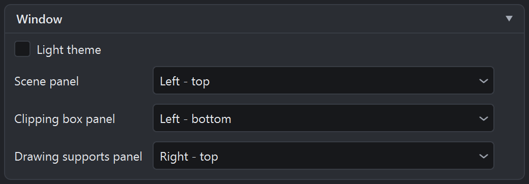
- Light theme
Interface in light colors: panels, menus, lists and bars. The 3D view keeps its own background (Background color, under 3D interface).
- Scene panel · Clipping box panel · Drawing outputs panel
Position of each panel: left or right of the view, at the top, middle or bottom of its column. The layout is kept from one session to the next.
3D interface
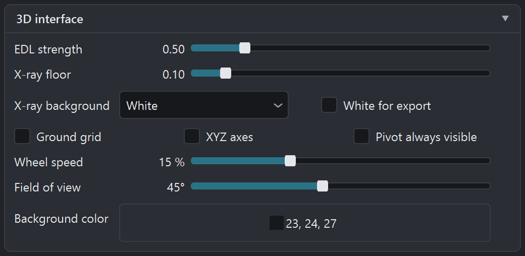
- X-ray floor
Share of the background the X-ray keeps where it is densest. At 0, the densest goes almost to black, or to white on a black background; at 1, nothing moves away from the background. Applied once to the finished image, on screen as in extraction.
- X-ray background
Background of the X-ray, on screen as on the sheets. White: the material darkens it, as on a radiograph. Black: it lightens it, in the manner of MeshLab. Default: white.
- White for export
Pure background for exported X-rays: pure white, or pure black with a black background, instead of the orthoimage background. The screen keeps its own background. Unchecked by default.
- Pivot always visible
Keeps the rotation-center marker always visible. Unchecked, it only shows for two seconds after a double-click.
- Wheel speed
Distance traveled per wheel notch, as a fraction of the distance to the surface under the cursor. The on-screen motion thus stays the same, near or far.
- Field of view
Lens aperture, measured on the height of the image. 20° gives a telephoto effect, close to a drawing plate; 80° a wide angle, handy in a narrow room but with stronger perspective. The framing does not change when switching to orthographic projection.
- Background color
Background tint of the 3D view: a very dark, slightly bluish gray by default. It does not affect the orthoimage background (Image background).
3D mouse
- Flight speed
Movement speed with a 3D mouse, as a percentage of the factory speed. At 100 %, the cap pushed all the way covers three tenths of the scene radius per second, about three meters per second in a house.
Point cloud
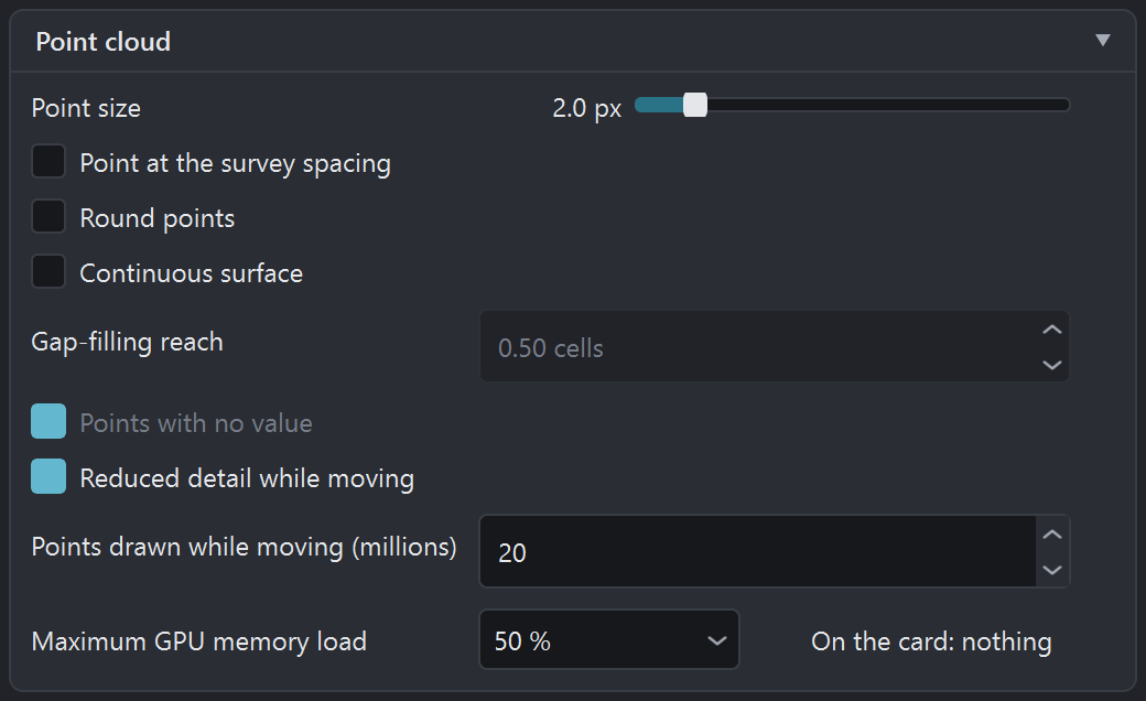
- Point size
Display size of the points, in pixels, with a minimum of one pixel.
- Point at the survey spacing
Point size set to the survey spacing rather than to a fixed number of pixels, as in the orthoimages: the screen shows what the extraction will deliver. The size then follows the zoom and the distance.
- Continuous surface
Fills in, on screen, the gaps between points, as if the cloud were a surface. The sky around a silhouette and openings wider than the reach stay empty.
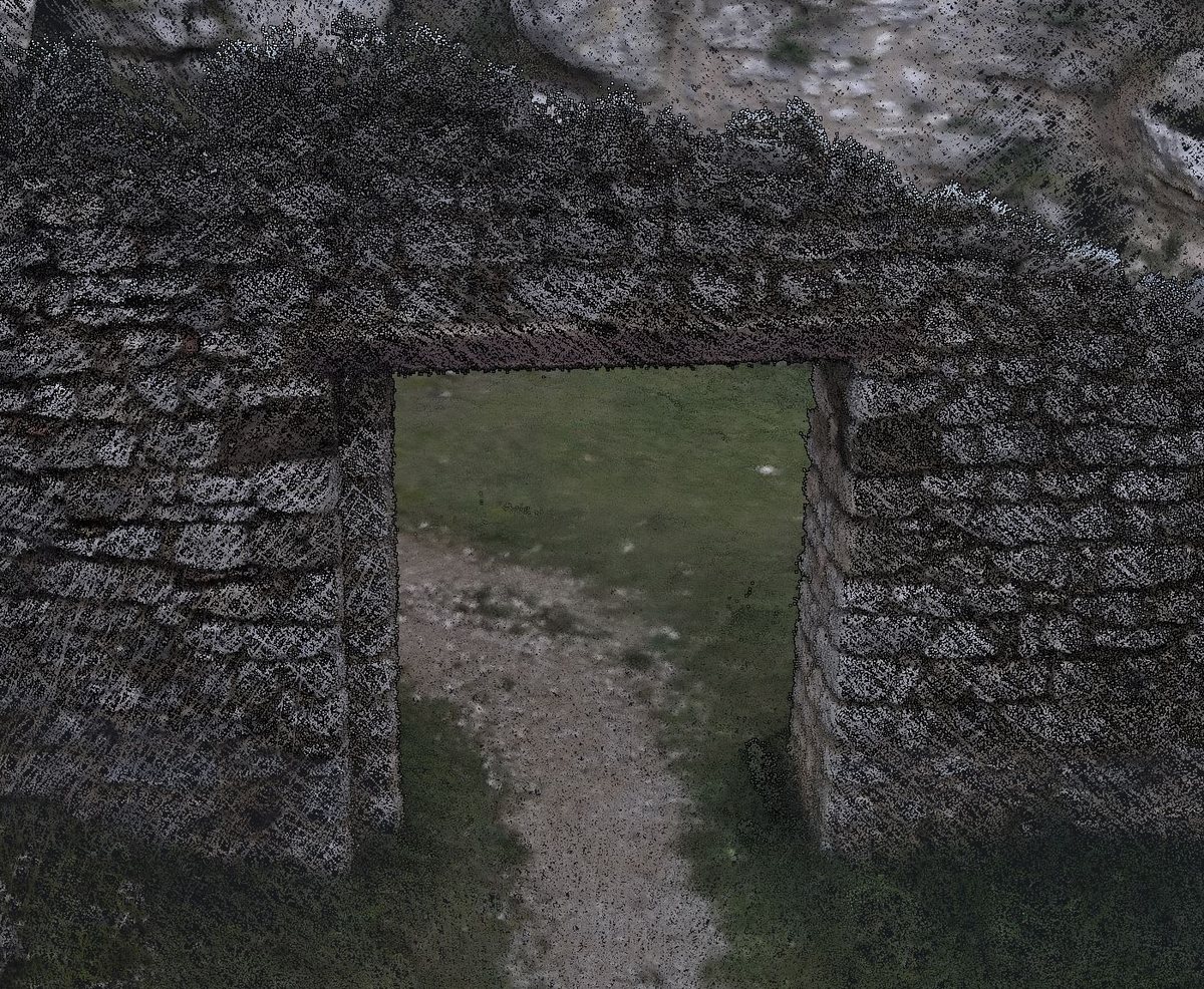
Off 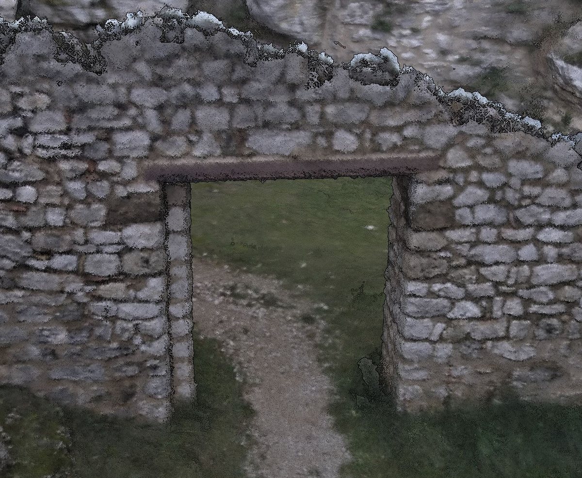
On - Gap-filling reach
Maximum distance to look for a neighboring point, in survey cells. A hole smaller than this reach is filled.
- Points with no value
Shows the points whose computed field has no value, where the neighborhood was too sparse for the computation. Checked, they show in the flat tint; unchecked, they disappear from the image. The box is only active if the current coloring contains any.
- Reduced detail while moving
While the view moves, only part of the cloud is drawn; the whole cloud comes back as soon as the view stops. Without this, a cloud of several hundred million points would freeze the window.
- Points drawn while moving (millions)
Maximum number of points drawn during a movement, in millions, all clouds together. Count about one millisecond per million: 20 million fit in a 21 ms frame.
- Maximum GPU memory load
Share of the graphics card memory reserved for point clouds, all clouds together. A point takes 16 bytes: 100 million points make 1.6 GB.
A cloud larger than this share sends only an even sample to the card. Sectioning, measurements and orthoimages always use the whole cloud.
3DGS models
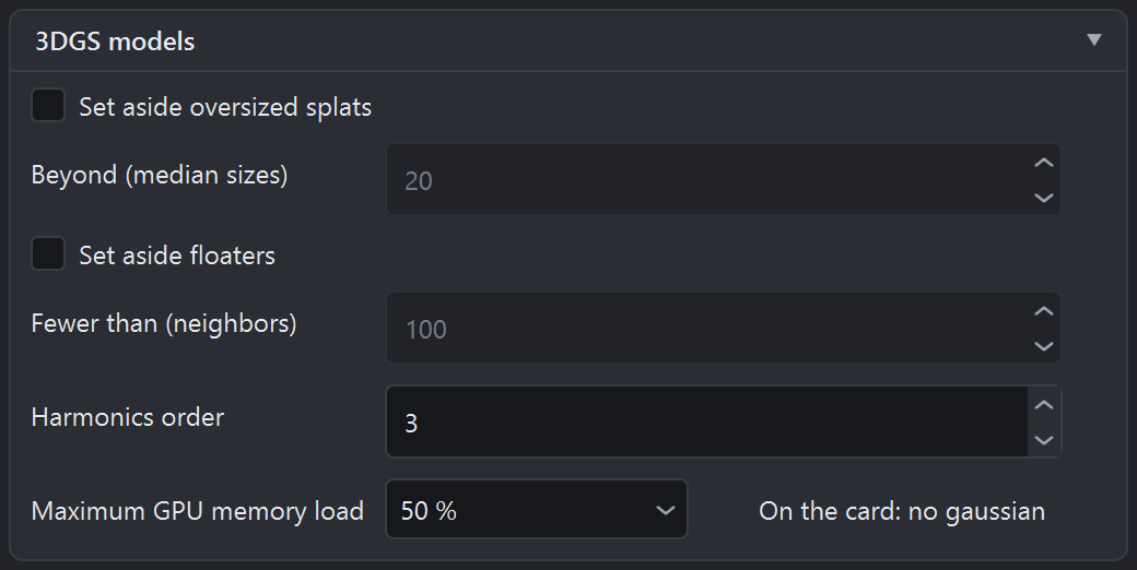
- Set aside oversized splats
Hides abnormally large splats, which the reconstruction places where it saw no surface: sky, background, the gap between two passes. Few in number, they still veil the view. Applies on screen, to orthoimages and to the PLY export.
- Beyond (median sizes)
Size threshold, in multiples of the median splat size. At 20, about one splat in ten thousand is set aside on a typical capture.
- Set aside floaters
Hides isolated splats, lost far from any surface: reconstruction floaters, clouds in the sky. The computation takes a few seconds for forty million splats. Applies on screen, to orthoimages and to the PLY export.
- Fewer than (neighbors)
Number of neighbors below which a splat counts as a floater. A surface has thousands.
- Harmonics order
Level of detail of the color changes with the viewing angle, such as reflections and highlights. 0: base color only; 3: everything the file contains. Applies at once, on screen as in orthoimages.
- Maximum GPU memory load
Share of the graphics card memory reserved for 3DGS models. A splat takes 69 to 189 bytes depending on its harmonics: ten million splats make 0.7 to 1.9 GB.
A model that is too large is loaded according to the view: every splat up close, the most visible ones in the distance.
Objects

- Uniform color
Tint of the models displayed without their colors: meshes without texture, and clouds in Uniform mode. The same tint serves both, so that a mesh and a cloud do not read as two different kinds of object.
Light gray, slightly bluish, by default. Textured OBJ files are not affected.
Mesh
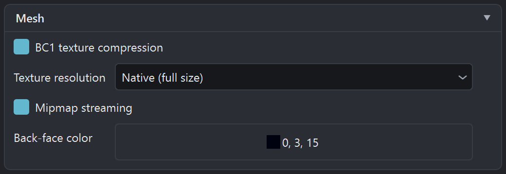
- BC1 texture compression
Compresses textures while loading: same resolution, about eight times less video memory. Takes effect on the next load.
- Texture resolution
Maximum texture resolution at load time. Takes effect on the next load.
- Mipmap streaming
Loads textures according to the view: only the levels of detail needed stay in video memory. The others wait in main memory and come back as you move closer.
- Back-face color
Tint of the faces seen from behind, on meshes and oriented clouds. Nearly black by default, to mark holes without catching the eye.
Drawing outputs
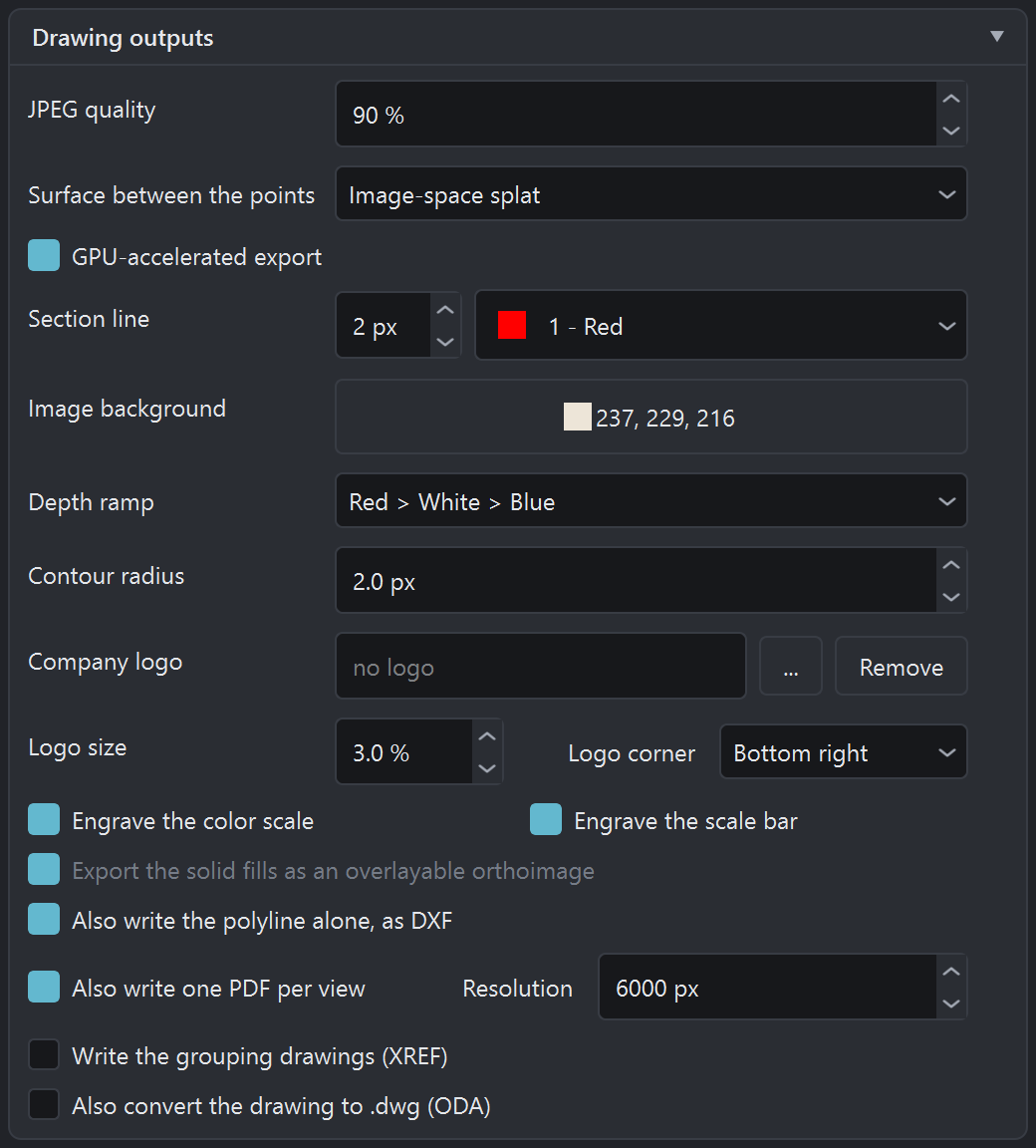
- JPEG quality
Compression quality of the JPEG orthoimages.
- Surface between the points
Method used to fill the space between cloud points in orthoimages:
- Image-space splat (default): no holes, and the best at following a survey of varying density;
- Weighted splatting (MeshLab): eight times faster, to produce a series; silhouettes spill over a little more;
- Discs at the sampling step: the method of versions up to 0.35.0, to redo an old plate identically;
- None: the raw survey, holes included, to judge its density before delivery.
No effect on meshes, X-ray or the depth map.
- GPU-accelerated export
Runs the stripping, filling and shading of point cloud images on the NVIDIA graphics card (CUDA) instead of the processor. The image comes out byte-for-byte identical; only the time changes: 19 s instead of 270 on a 32,000 pixel view. Checked by default.
- Section line width
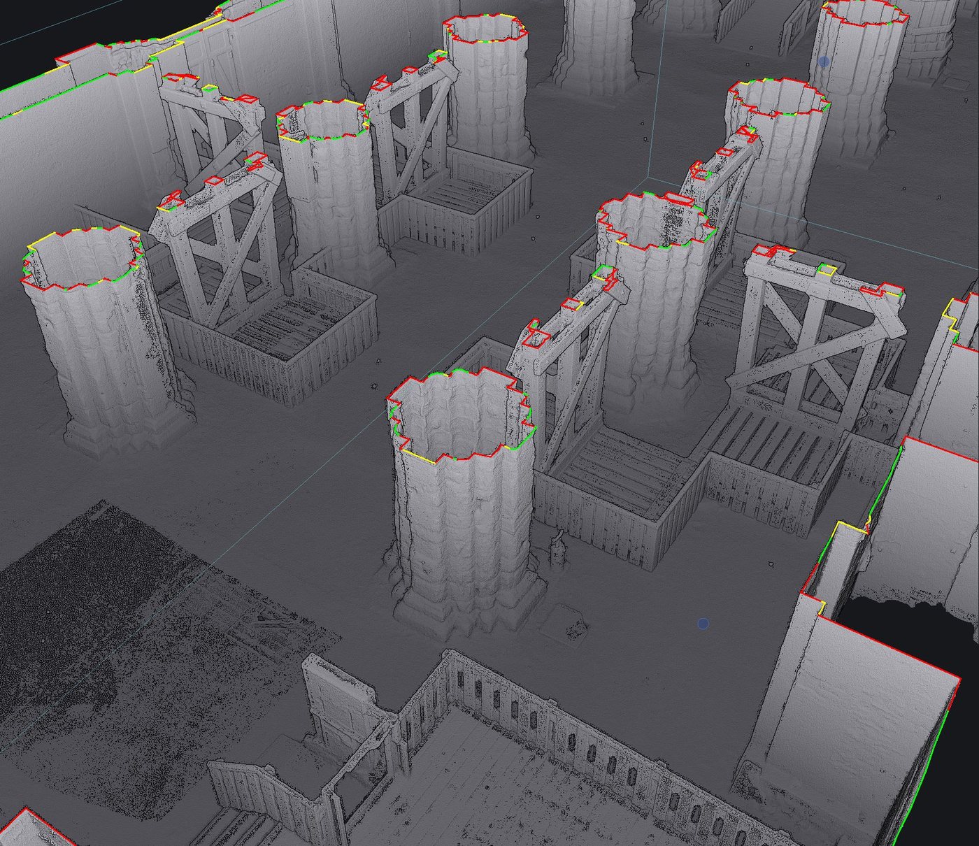
Thickness of the section line on screen, in pixels, constant whatever the zoom.
- Section line color
AutoCAD color of the polyline, by its index number, the same on screen and in the drawing. Three special values:
- 1: red, the color of the Cyclone 3DR chain;
- 0: color by the confidence index of the line (red below 0.5, yellow up to 0.75, green above), on three separate layers;
- -1: no line; no polyline is computed, which speeds up the export of clouds.
- Image background
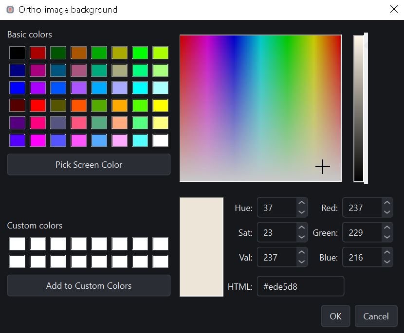
Color of the empty pixels of the orthoimages. By default, the cream tint of the 3DR chain (237, 229, 216), which stands out from the light surfaces of the model, both to the eye and to a threshold.
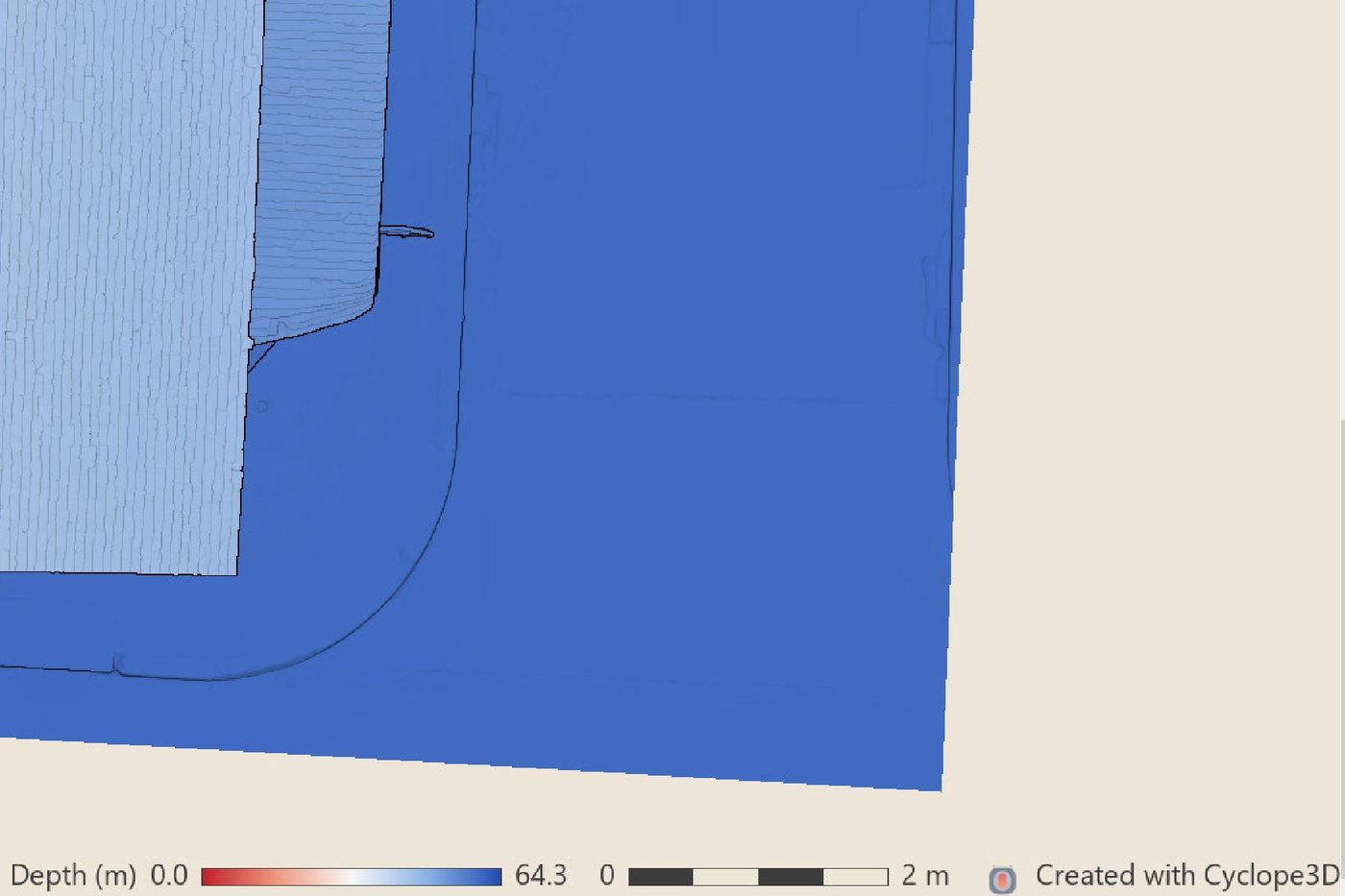
- Depth ramp
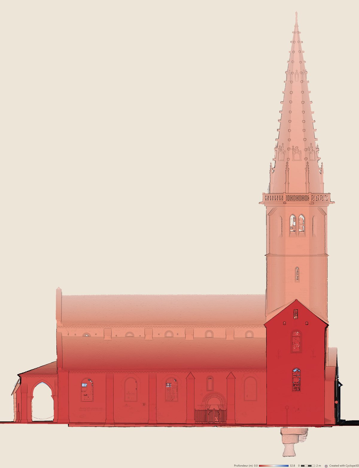
Palette of the depth maps. By default Red > White > Blue: red closest to the view plane, blue furthest.
- Contour radius
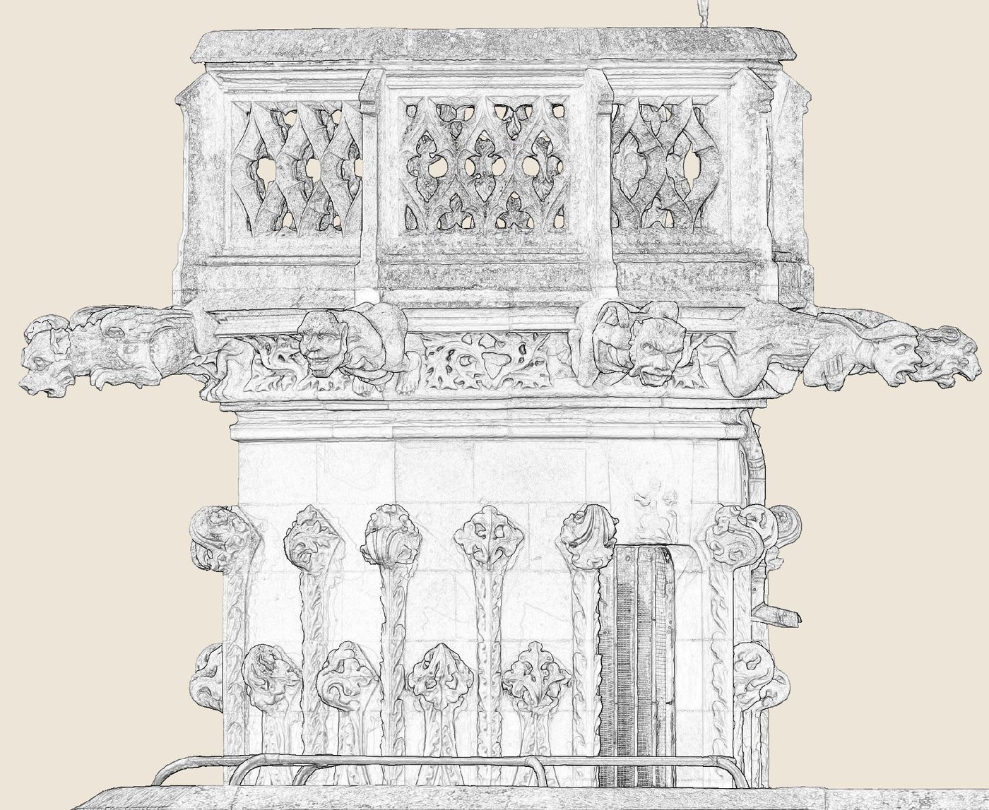
Thickness of the line in contour orthoimages, in pixels. Larger, the line thickens and gradients turn gray; smaller, only sharp edges remain.
- Company logo
Image burnt into a corner of every delivered orthoimage, followed by the mark “Created with Cyclope3D”. Without a logo, nothing is burnt in.
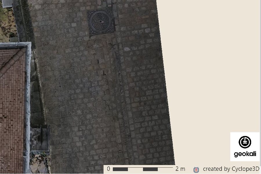
- Remove the logo
Removes the logo: the next orthoimages come out with neither logo nor mark.
- Logo size
Height of the logo, as a percentage of the image height: it thus keeps the same place on the plate whatever the resolution. The Cyclope3D mark stays at 1 %.
- Logo corner
Corner of the image where the logo, the scale bar and the color scale go.
- Engrave the color scale
Burns into the image the ramp that was used, with its bounds in meters. Without it, a delivered depth map does not say which distances its colors stand for. Concerns images whose color carries a value, currently the depth map.
- Engrave the scale bar
Burns a graduated scale bar of round length (20 cm, 50 cm, 1 m, 2 m, 5 m…) into every image.
- Export the solid fills as an overlayable orthoimage
Exports the solid fills, that is, the inside of the walls cut by the view plane, as a separate image: a transparent PNG, on its own layer, which can be turned on or off in the drawing. Unchecked, the fill is blended into the texture and flat-color images.
Solid fills are only delivered if Back faces tinted is checked.
- Also write the polyline alone, as DXF
Writes a second file,
<view>_polyline.dxf, containing only the section line: to lay it over an existing plan, or to send it without the images. DXF R12 format, readable by every program.- Also write one PDF per view
Writes one PDF per view, assembling the drawing's layers on one page: base map, solid fills and the section line as vectors. The other representations and the linked inverse plan are included, turned off.
- PDF resolution
Longest side of the images in the PDF, in pixels. Beyond it, images are scaled down; the drawing and the delivered images keep their full resolution.
- Write the grouping drawings (XREF)
Creates, at the root of the output folder, one drawing per family (plans; elevations and sections) that calls the other drawings as external references (XREF). Each view arrives on its own layer: the ground floor, the upper floor and the roofs can thus be stacked.
No image is duplicated, and a change to a drawing shows in the grouping. Two position files, one for plans and one for elevations and sections, come with them.
- Also convert the drawing to .dwg (ODA)
Adds a .dwg version of each drawing, next to the DXF, converted by the free Open Design Alliance tool. AutoCAD 2007 format, readable by every recent version.
Menus
File menu
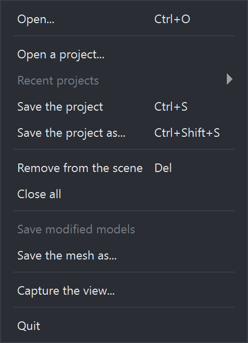
Opens an .extracts project: its views, their frames and the output settings replace those in the list. Same command as the Open a project… button of the Drawing outputs panel.
Saves the project to a new .extracts file, whose name and folder are asked for every time (Ctrl+Shift+S). Save the project (Ctrl+S) rewrites the current project without asking.
Saves the models changed during the session and not yet written: cuts kept in memory, meshes with flipped faces. Each one is written to a new file next to the original; nothing is ever overwritten.
Exports the selected mesh as OBJ, in its current state, for example after flipped faces have been corrected. The MTL file and the textures are copied alongside: the export is complete and can be moved.
Saves the 3D view as an image, at the resolution you want, with the same framing as on screen.
View menu
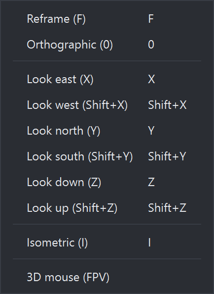
Switches between perspective and orthographic projection. In orthographic, parallel lines stay parallel and a measurement is worth the same everywhere: it is the projection of drawing plates and extractions.
View facing east: it shows the west facade.
View facing west: it shows the east facade.
View facing north: it shows the south facade.
View facing south: it shows the north facade.
View from above: the plan view.
View from below: the ceiling view.
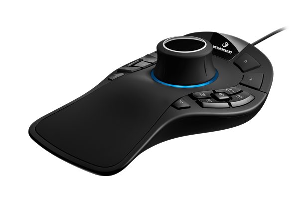
Drives the view with a 3Dconnexion 3D mouse, flying in first person: push the cap to move forward, pull it to move back, twist or tilt it to turn the gaze.
Analysis menu
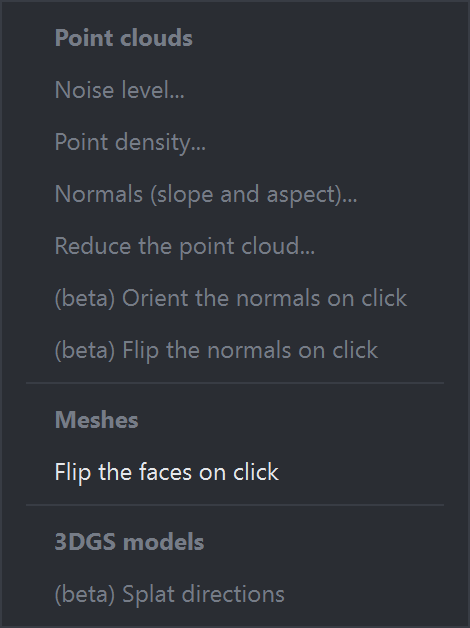
Measures the thickness of the point sheet, point by point, to assess the noise of a survey. Point clouds only.
Computes the density in points per square meter, from the 64 nearest neighbors of each point. Nothing to set: the neighborhood widens by itself in sparse areas. Point clouds only.
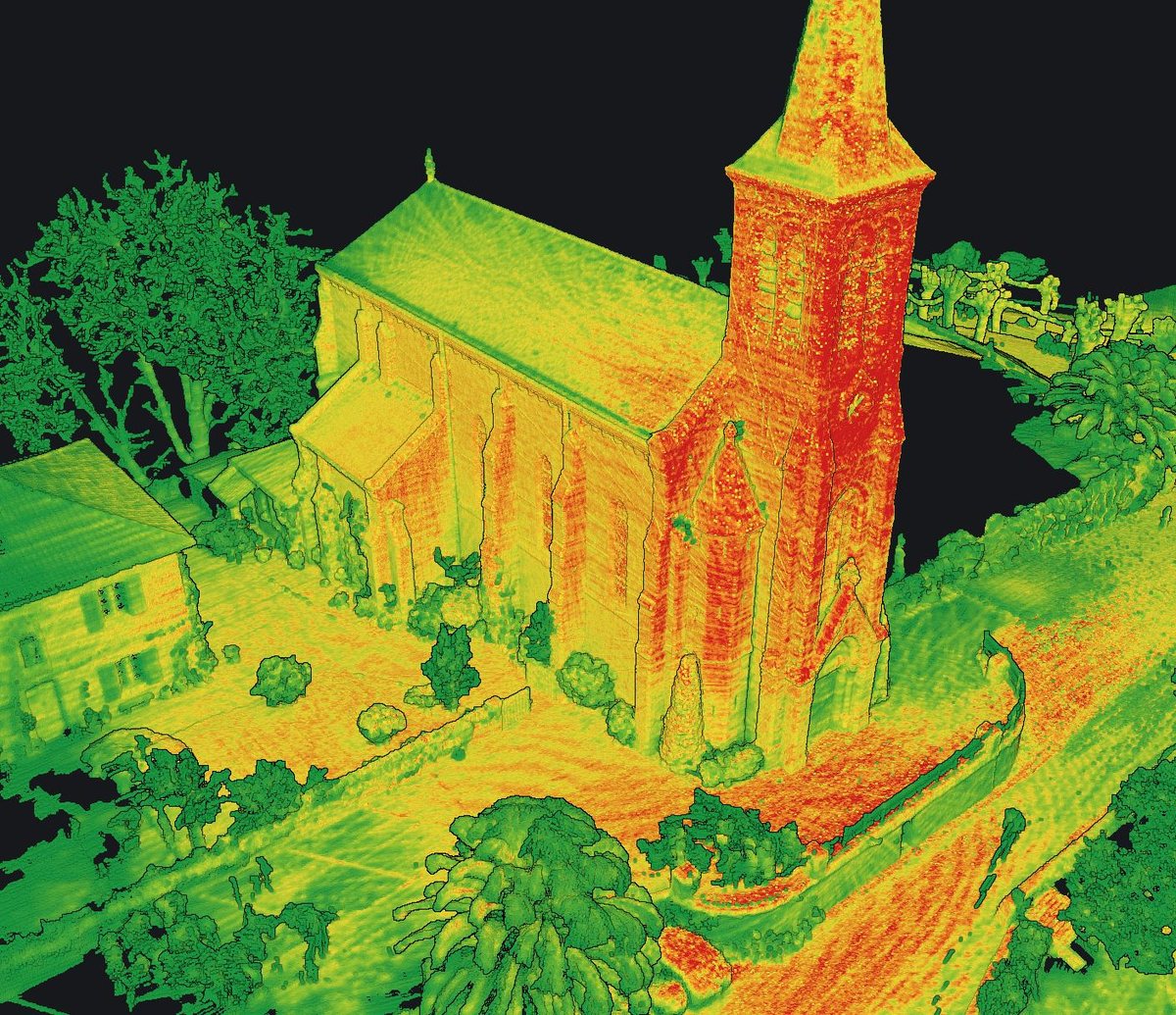
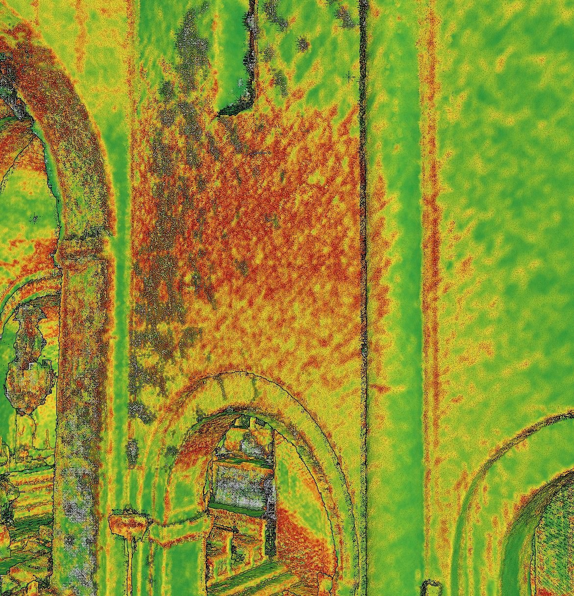
Computes the normal of each point, which gives two colorings: slope (0 to 90°) and aspect (0 to 180°). A third one, Normals, shows the normal in red, green and blue. Clouds only: a mesh already has its normals.
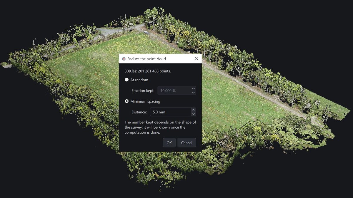
Reduces the number of points, written to a new LAS file and added to the scene:
- At random: keeps a share of the points, preserving the density differences of the survey;
- At minimum spacing: no two kept points closer than the requested distance (5 mm by default); the density becomes uniform.
Orients the normals of a cloud from a clicked point: the normal of that point is turned toward you, then the orientation spreads to the whole cloud.
Corrects the inside-out normals of a cloud, which show as patches of another tint in the middle of a wall. A click flips the whole zone up to its break lines; a second click undoes it. Esc releases the mouse.
Corrects the inside-out faces of a mesh, which show as patches of the back-face color. A click flips the whole zone up to its break edges; a second click undoes it. Esc releases the mouse.
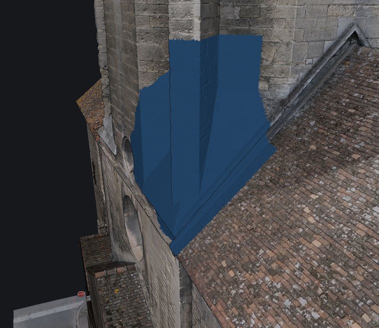
Before 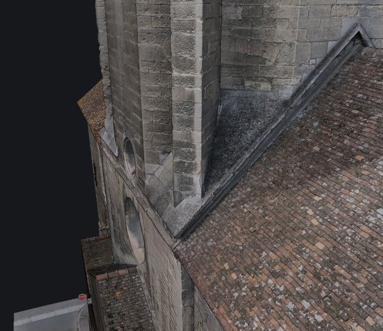
After Computes the side of each splat of the 3DGS models, the one the cameras saw it from: Inv. faces and Transparency use it. Applies to the selected models, or to all; about a minute for twenty million splats. Esc stops it.
? menu (help)
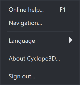
Opens this help page in the browser: workflows, panels and settings. Also with the F1 key and from the About box.
Reminder of the mouse gestures and keyboard shortcuts of the 3D view.
Interface language, French or English. The change is immediate.
Software version, contact and signed-in account.
Signs the account out on this computer, then closes the software. The license is checked at each startup.